Analytics 2013 Conference in Florida

Looking for case studies of data analytics or predictive analytics, or for Big Data applications?

You can hardly do better, on a first cut, than peruse the material now available from October’s Analytics 2013 Conference, held at the Hyatt Regency Hotel in Orlando, Florida.

Presented by SAS, dozens of presentations and posters from the Conference can be downloaded as zip files, unbundling as PDF files.

Download the conference presentations and poster presentations (.zip)

I also took an hour to look at the Keynote Presentation of Dr. Sven Crone of Lancaster University in the UK, now available on YouTube.

Crone, who also is affiliated with the Lancaster Centre for Forecasting, gave a Keynote which was, in places, fascinating, and technical and a little obscure elsewhere – worth watching if you time, or can run it in the background while you sort through your desk, for example.

A couple of slides caught my attention.

One segment gave concrete meaning to the explosion of data available to forecasters and analysts. For example, for electric power load forecasting, it used be the case that you had, perhaps, monthly total loads for the system or several of its parts, or perhaps daily system loads. Now, Crone notes the data to be modeled has increased by orders of magnitude, for example, with Smart Meters recording customer demand at fifteen minute intervals.

 Analytics13A1                      

Another part of Crone’s talk which grabbed my attention was his discussion of forecasting techniques employed by 300 large manufacturing concerns, some apparently multinational in scale. The following graph – which is definitely obscure by virtue of its use of acronyms for types of forecasting systems, like SOP for Sales and Operation Planning – highlights that almost no company uses anything except the simplest methods for forecasting, relying largely on judgmental approaches. This aligns with a survey I once did which found almost no utilities used anything except the simplest per capita forecasting approaches. Perhaps things have changed now.

Analytics13A1 Analytics13A2

Crone suggests relying strictly on judgment becomes sort of silly in the face of the explosion of information now available to management.

Another theme Crone spins in an amusing, graphic way is that the workhorses of business forecasting, such as exponential smoothing, are really products from many decades ago. He uses funny pics of old business/office environments, asking whether this characterizes your business today.

The analytic meat of the presentation comes with exposition of bagging and boosting, as well as creative uses for k-means clustering in time series analysis.

At which point he descends into a technical wonderland of complexity.

Incidentally, Analytics 2014 is scheduled for Frankfurt, Germany June 4-5 this coming Spring.

Watch here for my follow-on post on boosting time series.

Links January 16, 2014

Economic Outlook

Central Station: January Fed Taper on Track

Federal Reserve officials, including a strong supporter of their easy money policies, have so far brushed off the weak employment report as a blip in an otherwise strengthening economic recovery. This suggests they are likely to stick to their plan to gradually wind down their bond-buying program this year as the recovery picks up momentum…

“True, the December jobs report was disappointing,” said Chicago Fed President Charles Evans, who has been a champion of aggressive central bank efforts to spur stronger economic growth. But, he added, “the recent data on economic activity generally have been encouraging” and “importantly, the labor market has improved.”

He said the tentative plan to reduce the monthly bond buys in $10 billion increments “seems quite reasonable” and “it makes sense to continue that in January.

Atlanta Fed President Dennis Lockhart, a centrist on Fed policies, said Monday the December employment report hadn’t shaken his expectation that the central bank would stick to the taper plan.

Meanwhile two opponents of the bond-buying program, Dallas Fed President Richard Fisher and Philadelphia Fed President Charles Plosser indicated in separate speeches Tuesday they were all for winding it down.

Given that chorus, it appears probable Fed officials will trim their monthly bond purchases to $65 billion from $75 billion at their next policy meeting January 28-29 meeting. Now that tapering is under way, the bar for stopping the process seems quite high.

Big Data

Big Data systems are making a difference in the fight against cancer Open source, distributed computing tools speedup an important processing pipeline for genomics data

Big Data to increase e-tailer profits

As tablet and smartphone usage becomes more widespread, shopping online has become quicker and easier and the speed of delivery has become critical in the online fulfilment race.

The group of researchers, which includes Arne Strauss, Assistant Professor of Operational Research at Warwick Business School, propose an analytic approach that will predict when people want their shopping delivered depending on what delivery prices (or incentives such as discounts or loyalty points) are being quoted for different delivery time slots.

It takes into account accepted orders to date as well as orders that are still expected to come in….

The new approach was tested using real shopping data from a major e-grocer in the UK over a period of six months and generated a four per cent increase in profits on average in a simulation study, outperforming traditional delivery pricing policies.

Big Data and Data Science Books – A Baker’s Dozen – from Analytic Bridge

  1. Big Data: A Revolution That Will Transform How We Live, Work, and T…, by Viktor Mayer-Schonberger and Kenneth Cukier
  2. The Signal and the Noise: Why So Many Predictions Fail-but Some Don’t, by Nate Silver
  3. Predictive Analytics: The Power to Predict Who Will Click, Buy, Lie…, by Eric Siegel
  4. The Human Face of Big Data, by Rick Smolan and Jennifer Erwitt
  5. Data Science for Business: What you need to know about data mining …, by Foster Provost and Tom Fawcett
  6. The Black Swan: The Impact of the Highly Improbable, by Nassim Nicholas Taleb
  7. Competing on Analytics: The New Science of Winning, by Thomas H. Davenport and Jeanne G. Harris
  8. Super Crunchers: Why Thinking-by-Numbers is the New Way to Be Smart, by Ian Ayres
  9. Big Data Marketing: Engage Your Customers More Effectively and Driv…, by Lisa Arthur
  10. Journeys to Data Mining: Experiences from 15 Renowned Researchers, by Mohamed Medhat Gaber (editor)
  11. The Fourth Paradigm: Data-Intensive Scientific Discovery, by T.Hey, S.Tansley, and K.Tolle (editors)
  12. Seven Databases in Seven Weeks: A Guide to Modern Databases and the…, by Eric Redmond and Jim Wilson
  13. Data Mining And Predictive Analysis: Intelligence Gathering And Cri…, by Colleen McCue

Social Media

The History and Evolution of Social Media an Infographic (click to enlarge)

socialmediahistory

If you like this, there are many more infographics focusing on social media at https://www.pinterest.com/JuanCMejiaLlano/social-media-ingles/ – some in Spanish. Also check out Top 10 Infographics of 2013 [Daily Infographic].

Economics

Economics: Science, Craft, or Snake Oil? – nice, but sort of equivocating essay by Dani Rodrik from his new offices at the Princeton Institute for Advanced Studies. Answer – all of the above.

Origin and Importance of the Salesman in US – A piece of US business history and culture. I like this.

World Bank Economic Forecast

The World Bank issued its latest Global Economic Prospects report this week, basically offering up a forecast based on dynamics of (a) moderate increases in growth in the US and Europe (assuming no abrupt, but a gradual taper of QE), and (b) slowing, but stable growth in the developing world at a pace still about double that of the “developed” countries.

The story is, as with other macroeconomic forecasts issued recently by investment banks, that constraints, such as the fiscal drag on growth are being loosened, both in the US and in Europe. With currently low interest rates and continuing excess capacity, this suggests more rapid economic US and EU growth in 2014. Together with the still high average rates of growth in China and elsewhere, this suggests to the World Bank economists, that global growth will quicken in 2014.

Here is a World Bank spokesman with the basic story of the new Global Economic Prospects release.

And here are some of the specific numbers in the report (click to enlarge).

WBforecast

The Evolution of Kaggle

Kaggle is evolving in industry-specific directions, although it still hosts general data and predictive analytics contests.

“We liked to say ‘It’s all about the data,’ but the reality is that you have to understand enough about the domain in order to make a business,” said Anthony Goldbloom, Kaggle’s founder and chief executive. “What a pharmaceutical company thinks a prediction about a chemical’s toxicity is worth is very different from what Clorox thinks shelf space is worth. There is a lot to learn in each area.”

Oil and gas, which for Kaggle means mostly fracking wells in the United States, have well-defined data sets and a clear need to find working wells. While the data used in traditional oil drilling is understood, fracking is a somewhat different process. Variables like how long deep rocks have been cooked in the earth may matter. So does which teams are working the fields, meaning early-stage proprietary knowledge is also in play. That makes it a good field to go into and standardize.

(as reported in http://bits.blogs.nytimes.com/2014/01/01/big-data-shrinks-to-grow/?_r=0)

This December 2013 change of direction pushed out Jeremy Howard, Kaggle’s former Chief Data Scientist, who now says he is,

focusing on building new kinds of software that could better learn about the data it was crunching and offer its human owners insights on any subject.

“A lone wolf data scientist can still apply his knowledge to any industry,” he said. “I’m spending time in areas where I have no industrial knowledge and finding things. I’m going to have to build a company, but first I have to spend time as a lone wolf.”

A year or so ago, the company evolved into a service-provider with the objective of linking companies, top competitors and analytical talent, and the more than 100,000 data scientists who compete on its platform.

So Kaggle now features CUSTOMER SOLUTIONS ahead of COMPETITIONS at the head of its homepage, saying We’re the global leader in solving business challenges through predictive analytics. The homepage also features logos from Facebook GE, MasterCard, and NASA, as well as a link Compete as a data scientist for fortune, fame and fun ».

But a look at the competitions underway currently highlight the fact that just a few pay a prize now.

Kaggleactivecomps

Presumeably, companies looking for answers are now steered into the Kaggle network. The Kaggle Team numbers six analysts with experience in several industries, and the Kaggle Community includes scores of data and predictive analytics whizzes, many with “with multiple Kaggle wins.”

Here is a selection of Kaggle Solutions.

KaggleSolutions

This video gives you a good idea of the current focus of the company.

This is a big development in a way, and supports those who point to the need for industry-specific knowledge and experience to do a good job of data analytics.

The Problem of Many Predictors – Ridge Regression and Kernel Ridge Regression

You might imagine that there is an iron law of ordinary least squares (OLS) regression – the number of observations on the dependent (target) variable and associated explanatory variables must be less than the number of explanatory variables (regressors).

Ridge regression is one way to circumvent this requirement, and to estimate, say, the value of p regression coefficients, when there are N<p training sample observations.

This is very helpful in all sorts of situations.

Instead of viewing many predictors as a variable selection problem (selecting a small enough subset of the p explanatory variables which are the primary drivers), data mining operations can just use all the potential explanatory variables, if the object is primarily predicting the value of the target variable. Note, however, that ridge regression exploits the tradeoff between bias and variance – producing biased coefficient estimates with lower variance than OLS (if, in fact, OLS can be applied).

A nice application was developed by Edward Malthouse some years back. Malthouse used ridge regression for direct marketing scoring models (search and you will find a downloadable PDF). These are targeting models to identify customers for offers, so the response to a mailing is maximized. A nice application, but pre-social media in its emphasis on the postal service.

In any case, Malthouse’s ridge regressions provided superior targeting capabilities. Also, since the final list was the object, rather than information about the various effects of drivers, ridge regression could be accepted as a technique without much worry about the bias introduced in the individual parameter estimates.

Matrix Solutions for Ordinary and Ridge Regression Parameters

Before considering spreadsheets, let’s highlight the similarity between the matrix solutions for OLS and ridge regression. Readers can skip this section to consider the worked spreadsheet examples.

Suppose we have data which consists of N observations or cases on a target variable y and vector of explanatory variables x,

y1           x11         x12         ..             x1p

y2           x21         x22         ..             x2p

………………………………….

yN          xN1        xN2        ..             xNp


Here yi is the ith observation on the target variable, and xi=(xi1,xi2,..xip) are the associated values for p (potential) explanatory variables, i=1,2,..,N.

So we are interested in estimating the parameters of a relationship Y=f(X1,X2,..Xk).

Assuming f(.) is a linear relationship, we search for the values of k+1 parameters (β01,…,βp) such that  Σ(y-f(x))2 minimizes the sum of all the squared errors over the data – or sometimes over a subset called the training data, so we can generate out-of-sample tests of model performance.

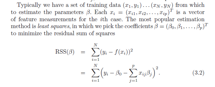
Following Hastie, Tibshirani, and Friedman, the Regression Sum of Squares (RSS) can be expressed,

LeastSquares

The solution to this least squares error minimization problem can be stated in a matrix formula,

β= (XTX)-1XTY

where X is the data matrix, Here XT denotes the transpose of the matrix X.

Now ridge regression involves creating a penalty in the minimization of the squared errors designed to force down the absolute size of the regression coefficients. Thus, the minimization problem is

RRminization

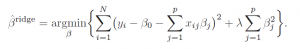
This also can be solved analytically in a closed matrix formula, similar to that for OLS –

βridge= (XTX-λІ)-1XTY

Here λ is a penalty or conditioning factor, and I is the identity matrix. This conditioning factor λ, it should be noted, is usually determined by cross-validation – holding back some sample data and testing the impact of various values of λ on the goodness of fit of the overall relationship on this holdout or test data.

Ridge Regression in Excel

So what sort of results can be obtained with ridge regression in the context of many predictors?

Consider the following toy example.

RRss

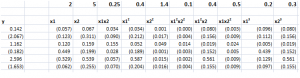
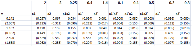
By construction, the true relationship is

y = 2x1 + 5x2+0.25x1x2+0.5x12+1.5x22+0.5x1x22+0.4x12x2+0.2x13+0.3x23

so the top row with the numbers in bold lists the “true” coefficients of the relationship.

Also, note that, strictly speaking, this underlying equation is not linear, since some exponents of explanatory variables are greater than 1, and there are cross products.

Still, for purposes of estimation we treat the setup as though the data come from ten separate explanatory variables, each weighted by separate coefficients.

Now, assuming no constant term and mean-centered data. the data matrix X is 6 rows by 10 columns, since there are six observations or cases and ten explanatory variables. Thus, the transpose XT is a 10 by 6 matrix. Accordingly, the product XTX is a 10 by 10 matrix, resulting in a 10 by 10 inverse matrix after the conditioning factor and identity matrix is added in to XTX.

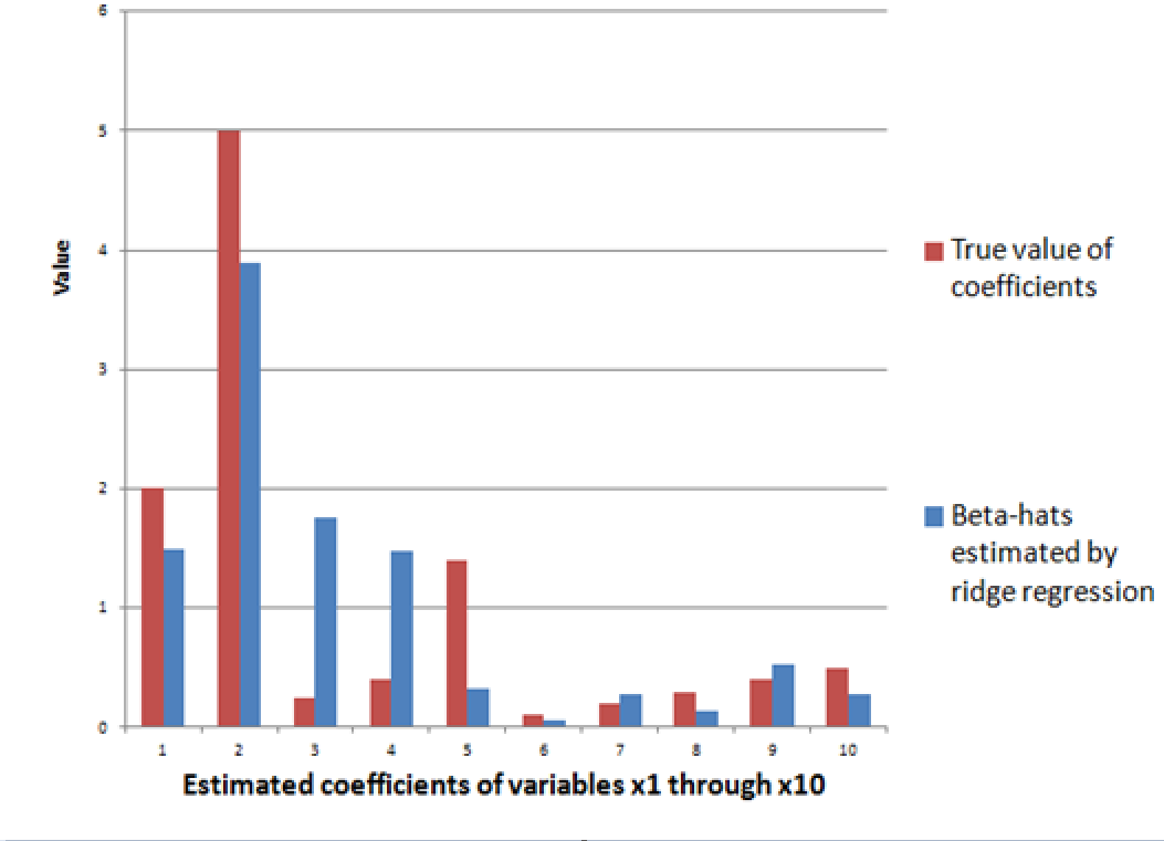
The ridge regression formula above, therefore, gives us estimates for ten beta-hats, as indicated in the following chart, using a λ or conditioning coefficient of .005.

RRestcomp

The red bars indicate the true coefficient values, and the blue bars are the beta-hats estimated by the ridge regression formula.

As you can see, ridge regression does get into the zone in terms of these ten coefficients of this linear expression, but with only 6 observations, the estimate is very approximate.

The Kernel Trick

Note that in order to estimate the ten coefficients by ordinary ridge regression, we had to invert a 10 by 10 matrix XTX. We also can solve the estimation problem by inverting a 6 by 6 matrix, using the kernel trick, whose derivation is outlined in a paper by Exertate.

The key point is that kernel ridge regression is no different from ordinary ridge regression…except for an algebraic trick.

To show this, we applied the ridge regression formula to the 6 by 10 data matrix indicated above, estimating the ten coefficients, using a λ or conditioning coefficient of .005. These coefficients broadly resemble the true values.

The above matrix formula works for our linear expression in ten variables, which we can express as

y = β1x1+ β2x2+… + β10x10

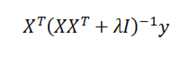
Now with suitable pre- and post-multiplications and resorting, it is possible to switch things around to arrive at another matrix formula,

Kerneltrick

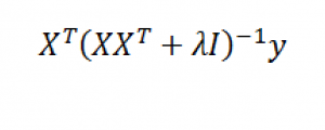
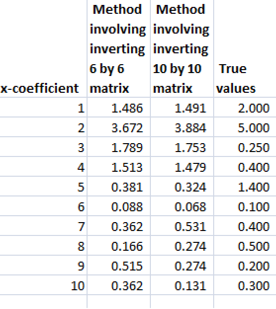
The following table shows beta-hats estimated by these two formulas are similar and compares them with the “true” values of the coefficients.

RRkerneltab

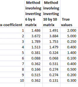
Differences in the estimates by these formulas relate strictly to issues at the level of numerical analysis and computation.

See also Exterkate et al “Nonlinear..” white paper.

Kernels

Notice that the ten variables could correspond to a Taylor expansion which might be used to estimate the value of a nonlinear function. This is important and illustrates the concept of a “kernel”.

Thus, designating K = XXwe find that the elements of K can be obtained without going through the indicated multiplication of these two matrices. This is because K is a polynomial kernel.

The second matrix formula listed just above involves inverting a smaller matrix, than the original formula – in our example, a 6 by 6, rather than a 10 by 10 matrix. This does not seem like a big deal with this toy example, but in Big Data and data mining applications, involving matrices with hundreds or thousands of rows and columns, the reduction in computation burden can be significant.

Summing Up

There is a great deal more that can be said about this example and the technique in general. Two big areas are (a) arriving at the estimate of the conditioning factor λ and (b) discussing the range of possible kernels that can be used, what makes a kernel a kernel, how to generate kernels from existing kernels, where Hilbert spaces come into the picture, and so forth.

But perhaps the important thing to remember is that ridge regression is one way to pry open the problem of many predictors, making it possible to draw on innumerable explanatory variables regardless of the size of the sample (within reason of course). Other techniques that do this include principal components regression and the lasso.

Predicting the S&P 500 or the SPY Exchange-Traded Fund

By some lights, predicting the stock market is the ultimate challenge. Tremendous resources are dedicated to it – pundits on TV, specialized trading programs, PhD’s doing high-end quantitative analysis in hedge funds. And then, of course, theories of “rational expectations” and “efficient markets” deny the possibility of any consistent success at stock market prediction, on grounds that stock prices are basically random walks.

I personally have not dabbled much in forecasting the market, until about two months ago, when I grabbed a bunch of data on the S&P 500 and tried some regressions with lags on S&P 500 daily returns and daily returns from the VIX volatility index.

What I discovered is completely replicable, and also, so far as I can see, is not widely known.

An autoregressive time series model of S&P 500 or SPY daily returns, built with data from 1993 to early 2008, can outperform a Buy & Hold strategy initiated with out-of-sample data beginning January 2008 and carrying through to recent days.

Here is a comparison of cumulative gains from a Buy & Hold strategy initiated January 23, 2008 with a Trading Strategy informed by my autoregressive (AR) model.

TradingStrategy1

So, reading this chart, investing $1000 January 23, 2008 and not touching this investment leads to cumulative returns of $1586.84 – that’s the Buy & Hold strategy.

The AR trading model, however, generates cumulative returns over this period of $2097.

The trading program based on the autoregressive model I am presenting here works like this. The AR model predicts the next day return for the SPY, based on the model coefficients (which I detail below) and the daily returns through the current day. So, if there is an element of unrealism, it is because the model is based on the daily returns computed on closing values day-by-day. But, obviously, you have to trade before the closing bell (in standard trading), so you need to use a estimate of the current day’s closing value obtained very close to the bell, before deciding whether to invest, sell, or buy SPY for the next day’s action.

But basically, assuming we can do this, perhaps seconds before the bell, and come close to an estimate of the current day closing price – the AR trading program is to buy SPY if the next day’s return is predicted to be positive – or if you currently hold SPY, to continue holding it. If the next day’s return is predicted to be negative, you sell your holdings.

It’s as simple as that.

So the AR model predicts daily returns on a one-day-ahead basis, using information on daily returns through the current trading day, plus the model coefficients.

Speaking of which, here are the coefficients from the Matlab “printout.”

MatlabTM1

There are a couple of nuances here. First, these parameter values do not derive from an ordinary least squares (OLS) regression. Instead, they are produced by maximum likelihood estimation, assuming the underlying distribution is a t-distribution (not a Gaussian distribution).

The use of a t-distribution, the idea of which I got to some extent from Nassim Taleb’s new text-in-progress mentioned two posts ago, is motivated by the unusual distribution of residuals of an OLS regression of lagged daily returns.

The proof is in the pudding here, too, since the above coefficients work better than ones developed on the (manifestly incorrect) assumption that the underlying error distribution is Gaussian.

Here is a graph of the 30-day moving averages of the proportion of signs of daily returns correctly predicted by this model.

TPproportions

Overall, about 53 percent of the signs of the daily returns in this out-of-sample period are predicted correctly.

If you look at this graph, too, it’s clear there are some differences in performance over this period. Thus, the accuracy of the model took a dive in 2009, in the depths of the Great Recession. And, model performance achieved significantly higher success proportions in 2012 and early 2013, perhaps related to markets getting used to money being poured in by the Fed’s policies of quantitative easing.

Why This AR Model is Such a Big Deal

I find it surprising that a set of fixed coefficients applied to the past 30 values of the SPY daily returns continue to predict effectively, months and years after the end of the in-sample values.

And, I might add, it’s not clear that updating the AR model always improves the outcomes, although I can do more work on this and also on the optimal sample period generally.

Can this be a matter of pure chance? This has to be considered, but I don’t think so. Monte Carlo simulations of randomized trading indicate that there is a 95 percent chance or better than returns of $2097 in this period are not due to chance. In other words, if I decide to trade on a day based on a flip of a fair coin, heads I buy, tails I sell at the end of the day, it’s highly unlikely I will generate cumulative returns of $2097, given the SPY returns over this period.

The performance of this trading model holds up fairly well through December of last year, but degrades some in the first days of 2014.

I think this is a feather in the cap of forecasting, so to speak. Also, it seems to me that economists promoting ideas of market efficiency and rational expectations need to take these findings into account. Everything is extant. I have provided the coefficients. You can get the SPY daily return values from Yahoo Finance. You can calculate everything yourself to check. I’ve done this several times, slightly differently each time. This time I used Matlab, and its arima estimation procedures work well.

I’m not quite sure what to make of all this, but I think it’s important. Naturally, I am extending these results in my personal model-building, and I can report that extensions are possible. At the same time, no extension of this model I have seen achieves more than nearly 60 percent accuracy in predicting the direction of change or sign of the daily returns, so you are going to lose money sometimes applying these models. Day-trading is a risky business.

Links – January 11, 2014

Sober Looks at the US Economy and Social Setup

Joseph Stiglitz is calling the post-2008 “recovery” period The Great Malise

Yes, we avoided a Great Depression II, but only to emerge into a Great Malaise, with barely increasing incomes for a large proportion of citizens in advanced economies. We can expect more of the same in 2014. In the United States, median incomes have continued their seemingly relentless decline; for male workers, income has fallen to levels below those attained more than 40 years ago. Europe’s double-dip recession ended in 2013, but no one can responsibly claim that recovery has followed. More than 50% of young people in Spain and Greece remain unemployed.…Europe’s continuing stagnation is bad enough; but there is still a significant risk of another crisis in yet another eurozone country, if not next year, in the not-too-distant future. Matters are only slightly better in the US, where a growing economic divide – with more inequality than in any other advanced country – has been accompanied by severe political polarization. …growth will remain anemic, barely strong enough to generate jobs for new entrants into the labor force. A dynamic tax-avoiding Silicon Valley and a thriving hydrocarbon sector are not enough to offset austerity’s weight. Thus, while there may be some reduction of the Federal Reserve’s purchases of long-term assets (so-called quantitative easing, or QE), a move away from rock-bottom interest rates is not expected until 2015 at the earliest…China’s decelerating growth had a significant impact on commodity prices, and thus on commodity exporters around the world. But China’s slowdown needs to be put in perspective: even its lower growth rate is the envy of the rest of the world, and its move toward more sustainable growth, even if at a somewhat lower level, will serve it – and the world – well in the long run. As in previous years, the fundamental problem haunting the global economy in 2013 remained a lack of global aggregate demand. This does not mean, of course, that there is an absence of real needs – for infrastructure, to take one example, or, more broadly, for retrofitting economies everywhere in response to the challenges of climate change. But the global private financial system seems incapable of recycling the world’s surpluses to meet these needs. And prevailing ideology prevents us from thinking about alternative arrangements…Maybe the global economy will perform a little better in 2014 than it did in 2013, or maybe not. Seen in the broader context of the continuing Great Malaise, both years will come to be regarded as a time of wasted opportunities.

On the 50th Anniversary of the War on Poverty, The Atlantic Monthly ran a first-rate article Poverty vs. Democracy in America. Full of pithy quotes and info, such as this about the emergence of an impoverished underclass

50 million strong—whose ranks have swelled since the Great Recession to the highest rate and number below the poverty line in nearly 50 years. Nearly half of them—20.5 million people, including each of the people mentioned above—are living in deep poverty on less than $12,000 per year for a family of four, the highest rate since record-keeping began in 1975. Add to that the hundred million citizens who are struggling to stay a few paychecks above the poverty line, and fully half the U.S. population is either poor or “near poor,” according to the Census Bureau.

 Economically speaking, their poverty entails a lack of decent-paying jobs and government supports to sustain a healthy life. With half of American jobs paying less than $33,000 per year and a quarter paying poverty-line wages of $22,000 or less, even as financial markets soar, people in the bottom fifth of the income distribution now command the smallest share of income—3.3 percent—since the government started tracking income breakdowns in the 1960s. Middle-wage jobs lost during the Great Recession are largely being replaced by low-wage jobs—when they are replaced at all—contributing to an 11 percent decline in real income for poor families since 1979. For the 27 million adults who are unemployed or underemployed and the 48 million people in working poor families who rely on some form of public support, means-tested government programs excluding Medicaid have remained essentially flat for the past 20 years, at around $1,000 per capita per year. Only unemployment insurance and food stamps have seen a marked increase in recent years, although both are currently under assault in Congress.

Indian and Chinese Space Programs

Here’s a beautiful picture of the Indian subcontinent, shot from space

 BdLAkorIgAAhv11                

This reminds me that India, currently, is sending an unmanned mission to Mars –  Mangalyaan. Mangalyaan left Earth orbit around the beginning of December 2013. December 11, it successfully completed a mid-course correction, and appears to be on its way to orbiting Mars by September of this year.

Not to be outdone, China landed an exploratory mission on Earth’s Moon in recent weeks. Here’s a pic taken by the “Jade Rabbit rover” vehicle brought there by the lander – I really like that name, “Jade Rabbit rover.”

Chinaspacemission

These missions both will be criticized as wasting valuable resources which could be used to deal with poverty and underdevelopment in the sponsoring countries. But I think it is more reasonable to consider all this under the heading leap-frogging – like countries which skip installing land lines for telephone service in favor of erecting lots of mobile communications towers. India and China are leapfrogging some stages of development, and may benefit from the science and technical challenges of space travel, which surely is part of the human future.

Here’s a relatively recent critique of China’s growing investment in science and technology which sounds suspiciously to me like sour grapes. It’s simple. Keep giving young people education in technical subjects with better and better science backing this up, and sheer numbers eventually will turn the tide. Inventors maybe from the interior provinces of China, neglected by the elite institutions, might come up with startling discoveries – if the US experience is any guide. A lot of the best US science and technology comes from relatively out-of-the-way places, state universities, industry labs, and then is snapped up by the elite institutions at the center.

2014 Outlook: Jan Hatzius Forecast for Global Economic Growth

Jan Hatzius is chief economist of Global Investment Research (GIR) at Goldman Sachs, and achieved notoriety with his early recognition of the housing bust in 2008.

Here he discusses the current outlook for 2014.

The outlook is fairly rosy, so it’s interesting Goldman just released “Where we worry: Risks to our outlook”, exerpted extensively at Zero Hedge.

Downside economic risks include:

1. Reduction in fiscal drag is less of a plus than we expect

2. Deleveraging obstacles continue to weigh on private demand

3. Less effective spare capacity leads to earlier wage/inflation pressure

4. Euro area risks resurface

5. China financial/credit concerns become critical


Predicting Financial Crisis – the Interesting Case of Nassim Taleb

Note: This is good post from the old series, and I am re-publishing it with the new citation to Taleb’s book in progress Hidden Risk and a new video.

———————————————–

One of the biggest questions is whether financial crises can be predicted in any real sense. This is a major concern of mine. I was deep in the middle of forecasting on an applied basis during 2008-2010, and kept hoping to find proxies to indicate, for example, when we were coming out of it, or whether it would “double-dip.”

Currently, as noted in this blog, a chorus of voices (commentators, analysts, experts) says that all manner of asset bubbles are forming globally, beginning with the US stock and the Chinese real estate markets.

But does that mean that we can predict the timing of this economic and financial crisis, or are we all becoming “Chicken Littles?”

What we want is well-described by Mark Buchanan, when he writes

The challenge for economists is to find those indicators that can provide regulators with reliable early warnings of trouble. It’s a complicated task. Can we construct measures of asset bubbles, or devise ways to identify “too big to fail” or “too interconnected to fail” institutions? Can we identify the architectural features of financial networks that make them prone to cascades of distress? Can we strike the right balance between the transparency needed to make risks evident, and the privacy required for markets to function?

And, ah yes – there is light at the end of the tunnel –

Work is racing ahead. In the U.S., the newly formed Office of Financial Research has published various papers on topics such as stress tests and data gaps — including one that reviews a list of some 31 proposed systemic-risk measures. The economists John Geanakoplos and Lasse Pedersen have offered specific proposals on measuring the extent to which markets are driven by leverage, which tends to make the whole system more fragile.

The Office of Financial Research (OFR) in the Treasury Department was created by the Dodd-Frank legislation, and it is precisely here Nassim Taleb enters the picture, at a Congressional hearing on formation of the OFR.

   untitled

Mr. Chairman, Ranking Member, Members of the Committee, thank you for giving me the opportunity to testify on the analytical ambitions and centralized risk-management plans of Office of Financial Research (OFR). I am here primarily as a practitioner of risk —not as an analyst but as a decision-maker, an eyewitness of the poor, even disastrous translation of risk research into practice. I spent close to two decades as a derivatives trader before becoming a full-time scholar and researcher in the areas of risk and probability, so I travelled the road between theory and practice in the opposite direction of what is commonly done. Even when I was in full-time practice I specialized in errors linked to theories, and the blindness from the theories of risk management. Allow me to present my conclusions upfront and in no uncertain terms: this measure, if I read it well, aims at the creation of an omniscient Soviet-style central risk manager. It makes us fall into the naive illusion of risk management that got us here —the same illusion has led in the past to the blind accumulation of Black Swan risks. Black Swans are these large, consequential, but unpredicted deviations in the eyes of a given observer —the observer does not see them coming, but, by some mental mechanism, thinks that he predicted them. Simply, there are limitations to our ability to measure the risks of extreme events and throwing government money on it will carry negative side effects. 1) Financial risks, particularly those known as Black Swan events cannot be measured in any possible quantitative and predictive manner; they can only be dealt with nonpredictive ways.  The system needs to be made robust organically, not through centralized risk management. I will keep repeating that predicting financial risks has only worked on computers so far (not in the real world) and there is no compelling reason for that to change—as a matter of fact such class of risks is becoming more unpredictable

A reviewer in the Harvard Business Review notes Taleb is a conservative with a small c. But this does not mean that he is a toady for the Koch brothers or other special interests. In fact, in this Congressional testimony, Taleb also recommends, as his point #3

..risks need to be handled by the entities themselves, in an organic way, paying for their mistakes as they go. It is far more effective to make bankers accountable for their mistakes than try the central risk manager version of Soviet-style central planner, putting hope ahead of empirical reality.

Taleb’s argument has a mathematical side. In an article in the International Journal of Forecasting appended to his testimony, he develops infographics to suggest that fat-tailed risks are intrinsically hard to evaluate. He also notes, correctly, that in 2008, despite manifest proof to the contrary, leading financial institutions often applied risk models based on the idea that outcomes followed a normal or Gaussian probability distribution. It’s easy to show that this is not the case for daily stock and other returns. The characteristic distributions exhibit excess kurtosis, and are hard to pin down in terms of specific distributions. As Taleb points out, the defining events that might tip the identification one way or another are rare. So mistakes are easy to make, and possibly have big effects.

But, Taleb’s extraordinary talent for exposition is on full view in an recent article How To Prevent Another Financial Crisis, coauthored with George Martin. The first paragraphs give us the conclusion,

We believe that “less is more” in complex systems—that simple heuristics and protocols are necessary for complex problems as elaborate rules often lead to “multiplicative branching” of side effects that cumulatively may have first order effects. So instead of relying on thousands of meandering pages of regulation, we should enforce a basic principle of “skin in the game” when it comes to financial oversight: “The captain goes down with the ship; every captain and every ship.” In other words, nobody should be in a position to have the upside without sharing the downside, particularly when others may be harmed. While this principle seems simple, we have moved away from it in the finance world, particularly when it comes to financial organizations that have been deemed “too big to fail.”

Then, the authors drive this point home with a salient reference –

The best risk-management rule was formulated nearly 4,000 years ago. Hammurabi’s code specifies: “If a builder builds a house for a man and does not make its construction firm, and the house which he has built collapses and causes the death of the owner of the house, that builder shall be put to death.” Clearly, the Babylonians understood that the builder will always know more about the risks than the client, and can hide fragilities and improve his profitability by cutting corners—in, say, the foundation. The builder can also fool the inspector (or the regulator). The person hiding risk has a large informational advantage over the one looking for it.

My hat’s off to Taleb. A brilliant example, and the rest of the article bears reading too.

While I have not thrown in the towel when it comes to devising metrics to signal financial crisis, I have to say that thoughts like Taleb’s probability argument occurred to me recently, when considering the arguments over extreme weather events.

Here’s a recent video.

Stock Market Bubble in 2014?

As of November, Janet Yellen, newly confirmed Chair of the US Federal Reserve Bank, doesn’t think so.

As reported in the Wall Street Journal MONEYBEAT, she said,

Stock prices have risen pretty robustly”… But looking at several valuation measures — she specifically cited equity-risk premiums — she said: “you would not see stock prices in territory that suggest…bubble-like conditions.”

Her reference to equity-risk premiums sent me to Aswath Damodaran’s webpage, which estimates this metric -basically the extra return investors demand to lure them into stocks and out of the safety of government bonds (in the Updated Data section). It’s definitely an implied value, so it’s hard to judge.

But what are some of the other Pro’s and Con’s regarding a stock market bubble?

Pros – There Definitely is a Bubble

The CAPE (cylically adjusted price earnings ratio) is approaching 2007 levels. This is a metric developed by Robert Shiller and, according to him, is supposed to be a longer term indicator, rather than something that can signal short-term movements in the market. At the same time, recent interviews, who recently shared a Nobel prize in economics, indicate Shiller is currently ‘most worried’ about ‘boom’ in U.S. stock market. Here is his CAPE indext (click this and the other charts here to enlarge).

shiller-cape

Several sector and global bubbles are currently reinforcing each other. When one goes pop, it’s likely to bring down the house of cards. In the words of Jesse Columbo, whose warnings in 2007 were prescient,

..the global economic recovery is actually what I call a “Bubblecovery” or a bubble-driven economic recovery that is driven by inflating post-2009 bubbles in China, emerging markets, Australia, Canada, Northern and Western European housing, U.S. housing, U.S. healthcare, U.S. higher education, global bonds, and tech (Web 2.0 and social media).

Margin debt, as reported by the New York Stock Exchange, is also at its all-time highs. Here’s a chart from Advisor Perspectives adjusting margin debt for inflation over a long period.

margindebt

Con – No Bubble Here

Stocks are the cheapest they have been in decades. This is true, as the chart below shows (based on trailing twelve month “as reported” earnings).

PEratios

The S&P 500, adjusted for inflation, has not reached the peaks of either 2000 or2007 (chart from All Start Charts)

10-7-13-spx-inf-adj

Bottom Line

I must confess, doing the research for the post, that I think the stock market in the US may have a ways to go, before it hits its peak this time. Dr. Yelen’s appointment suggests quantitative easing (QE) and low interest rates may continue for some time, before the Fed takes away the punch bowl. My guess is that markets are just waiting at this point to see whether this is, in fact, what is likely to happen,  or whether others in the Fed will exercise stronger control over policy, now Ben Bernacke is gone.

And, as seems probable, Yellen consolidates her control and signals continuation of current policies, then I suspect we will see some wild increases in asset values here and globally.