
I finally started learning R.
It’s a vector and matrix-based statistical programming language, a lot like MathWorks Matlab and GAUSS. The great thing is that it is free. I have friends and colleagues who swear by it, so it was on my to-do list.
The more immediate motivation, however, was my interest in Rob Hyndman’s automatic time series forecast package for R, described rather elegantly in an article in the Journal of Statistical Software.
This is worth looking over, even if you don’t have immediate access to R.
Hyndman and Exponential Smoothing
Hyndman, along with several others, put the final touches on a classification of exponential smoothing models, based on the state space approach. This facilitates establishing confidence intervals for exponential smoothing forecasts, for one thing, and provides further insight into the modeling options.
There are, for example, 15 widely acknowledged exponential smoothing methods, based on whether trend and seasonal components, if present, are additive or multiplicative, and also whether any trend is damped.
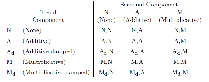
When either additive or multiplicative error processes are added to these models in a state space framewoprk, the number of modeling possibilities rises from 15 to 30.
One thing the Hyndman R Package does is run all the relevant models from this superset on any time series provided by the user, picking a recommended model for use in forecasting with the Aikaike information criterion.
Hyndman and Khandakar comment,
Forecast accuracy measures such as mean squared error (MSE) can be used for selecting a model for a given set of data, provided the errors are computed from data in a hold-out set and not from the same data as were used for model estimation. However, there are often too few out-of-sample errors to draw reliable conclusions. Consequently, a penalized method based on the in-sample t is usually better.One such approach uses a penalized likelihood such as Akaike’s Information Criterion… We select the model that minimizes the AIC amongst all of the models that are appropriate for the data.
Interestingly,
The AIC also provides a method for selecting between the additive and multiplicative error models. The point forecasts from the two models are identical so that standard forecast accuracy measures such as the MSE or mean absolute percentage error (MAPE) are unable to select between the error types. The AIC is able to select between the error types because it is based on likelihood rather than one-step forecasts.
So the automatic forecasting algorithm, involves the following steps:
1. For each series, apply all models that are appropriate, optimizing the parameters (both smoothing parameters and the initial state variable) of the model in each case.
2. Select the best of the models according to the AIC.
3. Produce point forecasts using the best model (with optimized parameters) for as many steps ahead as required.
4. Obtain prediction intervals for the best model either using the analytical results of Hyndman et al. (2005b), or by simulating future sample paths..
This package also includes an automatic forecast module for ARIMA time series modeling.
One thing I like about Hyndman’s approach is his disclosure of methods. This, of course, is in contrast with leading competitors in the automatic forecasting market space –notably Forecast Pro and Autobox.
Certainly, go to Rob J Hyndman’s blog and website to look over the talk (with slides) Automatic time series forecasting. Hyndman’s blog, mentioned previously in the post on bagging time series, is a must-read for statisticians and data analysts.
Quick Implementation of the Hyndman R Package and a Test
But what about using this package?
Well, first you have to install R on your computer. This is pretty straight-forward, with the latest versions of the program available at the CRAN site. I downloaded it to a machine using Windows 8 as the OS. I downloaded both the 32 and 64-bit versions, just to cover my bases.
Then, it turns out that, when you launch R, a simple menu comes up with seven options, and a set of icons underneath. Below that there is the work area.
Go to the “Packages” menu option. Scroll down until you come on “forecast” and load that.
That’s the Hyndman Forecast Package for R.
So now you are ready to go, but, of course, you need to learn a little bit of R.
You can learn a lot by implementing code from the documentation for the Hyndman R package. The version corresponding to the R file that can currently be downloaded is at
http://cran.r-project.org/web/packages/forecast/forecast.pdf
Here are some general tutorials:
http://cran.r-project.org/doc/contrib/Verzani-SimpleR.pdf
http://cyclismo.org/tutorial/R/
http://cran.r-project.org/doc/manuals/R-intro.html#Simple-manipulations-numbers-and-vectors
And here is a discussion of how to import data into R and then convert it to a time series – which you will need to do for the Hyndman package.
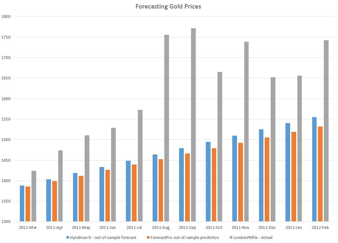
I used the exponential smoothing module to forecast monthly averages from London gold PM fix price series, comparing the results with a ForecastPro run. I utilized data from 2007 to February 2011 as a training sample, and produced forecasts for the next twelve months with both programs.
The Hyndman R package and exponential smoothing module outperformed Forecast Pro in this instance, as the following chart shows.
Another positive about the R package is it is possible to write code to produce a whole number of such out-of-sample forecasts to get an idea of how the module works with a time series under different regimes, e.g. recession, business recovery.
I’m still caging together the knowledge to put programs like that together and appropriately save results.
But, my introduction to this automatic forecasting package and to R has been positive thus far.