Category Archives: Big Data

Global Energy Forecasting Competitions

The 2012 Global Energy Forecasting Competition was organized by an IEEE Working Group to connect academic research and industry practice, promote analytics in engineering education, and prepare for forecasting challenges in the smart grid world. Participation was enhanced by alliance with Kaggle for the load forecasting track. There also was a second track for wind power forecasting.

Hundreds of people and many teams participated.

This year’s April/June issue of the International Journal of Forecasting (IJF) features research from the winners.

Before discussing the 2012 results, note that there’s going to be another competition – the Global Energy Forecasting Competition 2014 – scheduled for launch August 15 of this year. Professor Tao Hong, a key organizer, describes the expansion of scope,

GEFCom2014 (www.gefcom.org) will feature three major upgrades: 1) probabilistic forecasts in the form of predicted quantiles; 2) four tracks on demand, price, wind and solar; 3) rolling forecasts with incremental data update on weekly basis.

Results of the 2012 Competition

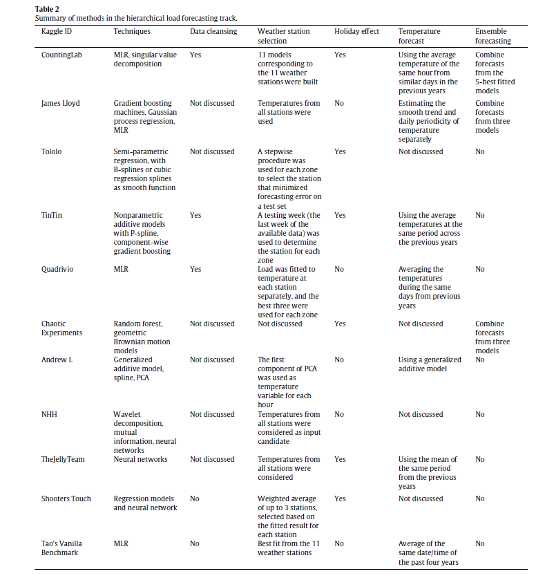
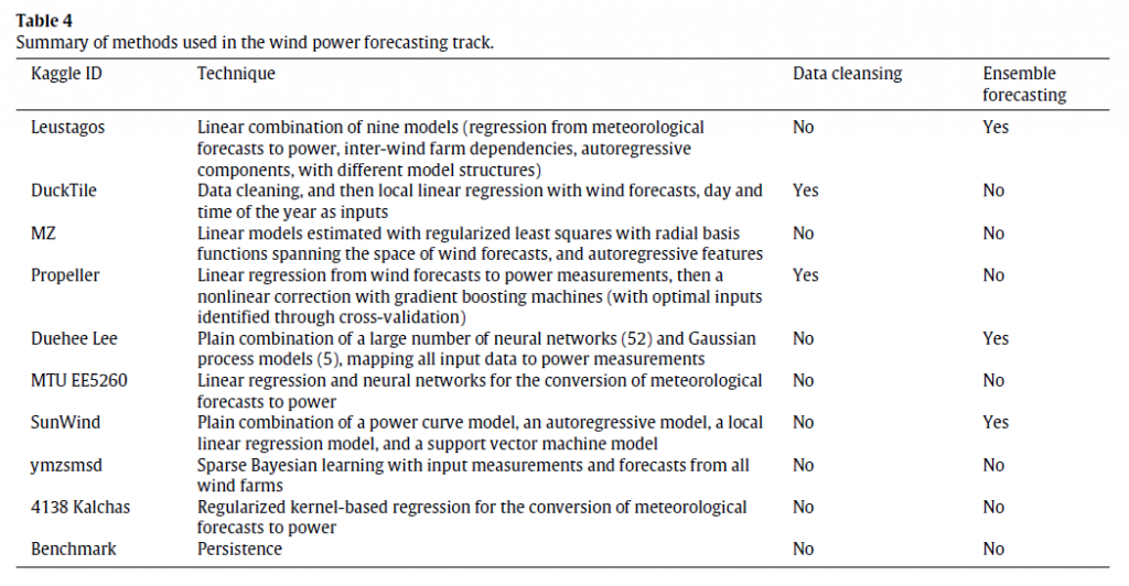
The IJF has an open source article on the competition. This features a couple of interesting tables about the methods in the load and wind power tracks (click to enlarge).

hload

The error metric is WRMSE, standing for weighted root mean square error. One week ahead system (as opposed to zone) forecasts received the greatest weight. The top teams with respect to WRMSE were Quadrivio, CountingLab, James Lloyd, and Tololo (Électricité de France).

wind

The top wind power forecasting teams were Leustagos, DuckTile, and MZ based on overall performance.

Innovations in Electric Power Load Forecasting

The IJF overview article pitches the hierarchical load forecasting problem as follows:

participants were required to backcast and forecast hourly loads (in kW) for a US utility with 20 zones at both the zonal (20 series) and system (sum of the 20 zonal level series) levels, with a total of 21 series. We provided the participants with 4.5 years of hourly load and temperature history data, with eight non-consecutive weeks of load data removed. The backcasting task is to predict the loads of these eight weeks in the history, given actual temperatures, where the participants are permitted to use the entire history to backcast the loads. The forecasting task is to predict the loads for the week immediately after the 4.5 years of history without the actual temperatures or temperature forecasts being given. This is designed to mimic a short term load forecasting job, where the forecaster first builds a model using historical data, then develops the forecasts for the next few days.

One of the top entries is by a team from Électricité de France (EDF) and is written up under the title GEFCom2012: Electric load forecasting and backcasting with semi-parametric models.

This is behind the International Journal of Forecasting paywall at present, but some of the primary techniques can be studied in a slide set by Yannig Goulde.

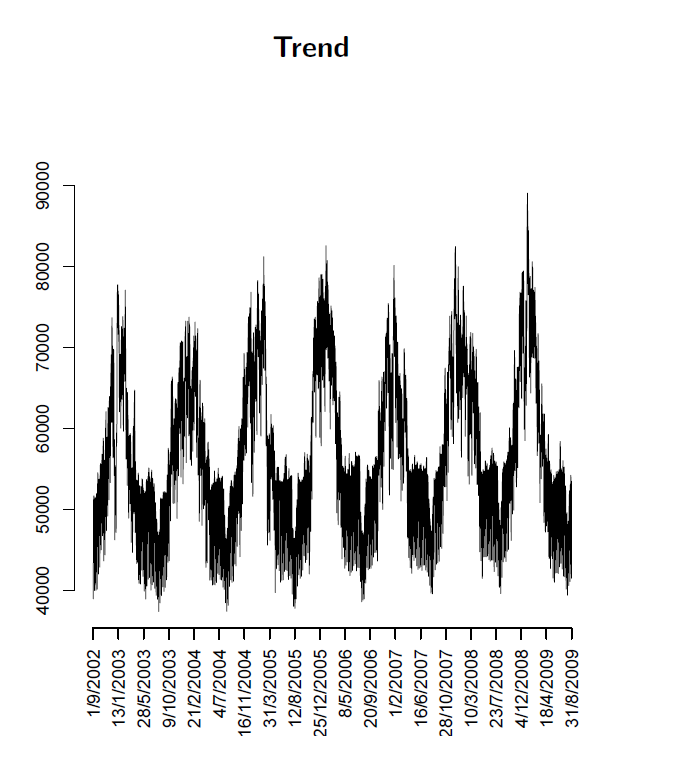
This is an interesting deck because it maps key steps in using semi-parametric models and illustrates real world system power load or demand data, as in this exhibit of annual variation showing the trend over several years.

trend

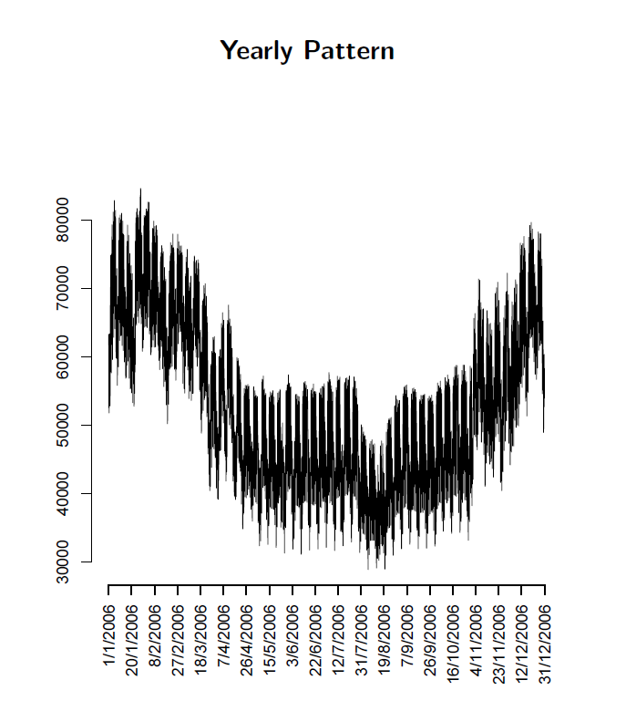
Or this exhibit showing annual variation.

annual

What intrigues me about the EDF approach in the competition and, apparently, more generally in their actual load forecasting, is the use of splines and knots. I’ve seen this basic approach applied in other time series contexts, for example, to facilitate bagging estimates.

So these competitions seem to provide solid results which can be applied in a real-world setting.

Top image from Triple-Curve

Data Analytics Reverses Grandiose Claims for California’s Monterey Shale Formation

In May, “federal officials” contacted the Los Angeles Times with advance news of a radical revision of estimates of reserves in the Monterey Formation,

Just 600 million barrels of oil can be extracted with existing technology, far below the 13.7 billion barrels once thought recoverable from the jumbled layers of subterranean rock spread across much of Central California, the U.S. Energy Information Administration said.

The LA Times continues with a bizarre story of how “an independent firm under contract with the government” made the mistake of assuming that deposits in the Monterey Shale formation were as easily recoverable as those found in shale formations elsewhere.

There was a lot more too, such as the information that –

The Monterey Shale formation contains about two-thirds of the nation’s shale oil reserves. It had been seen as an enormous bonanza, reducing the nation’s need for foreign oil imports through the use of the latest in extraction techniques, including acid treatments, horizontal drilling and fracking…

The estimate touched off a speculation boom among oil companies.

Well, I’ve combed the web trying to find more about this “mistake,” deciding that, probably, it was the analysis of David Hughes in “Drilling California,” released in March of this year, that turned the trick.

Hughes – a geoscientist working decades with the Geological Survey of Canada – utterly demolishes studies which project 15 billion barrels in reserve in the Monterey Formation. And he does this by analyzing an extensive database (Big Data) of wells drilled in the Formation.

The video below is well worth the twenty minutes or so. It’s a tour de force of data analysis, but it takes a little patience at points.

First, though, check out a sample of the hype associated with all this, before the overblown estimates were retracted.

Monterey Shale: California’s Trillion-Dollar Energy Source

Here’s a video on Hughes’ research in Drilling California

Finally, here’s the head of the US Energy Information Agency in December 2013, discussing a preliminary release of figures in the 2014 Energy Outlook, also released in May 2014.

Natural Gas 2014 Projections by the EIA’s Adam Sieminski

One question is whether the EIA projections eventually will be acknowledged to be affected by a revision of reserves for a formation that is thought to contain two thirds of all shale oil in the US.

Leading Indicators

One value the forecasting community can provide is to report on the predictive power of various leading indicators for key economic and business series.

The Conference Board Leading Indicators

The Conference Board, a private, nonprofit organization with business membership, develops and publishes leading indicator indexes (LEI) for major national economies. Their involvement began in 1995, when they took over maintaining Business Cycle Indicators (BCI) from the US Department of Commerce.

For the United States, the index of leading indicators is based on ten variables: average weekly hours, manufacturing,  average weekly initial claims for unemployment insurance, manufacturers’ new orders, consumer goods and materials, vendor performance, slower deliveries diffusion index,manufacturers’ new orders, nondefense capital goods, building permits, new private housing units, stock prices, 500 common stocks, money supply, interest rate spread, and an index of consumer expectations.

The Conference Board, of course, also maintains coincident and lagging indicators of the business cycle.

This list has been imprinted on the financial and business media mind, and is a convenient go-to, when a commentator wants to talk about what’s coming in the markets. And it used to be that a rule of thumb that three consecutive declines in the Index of Leading Indicators over three months signals a coming recession. This rule over-predicts, however, and obviously, given the track record of economists for the past several decades, these Conference Board leading indicators have questionable predictive power.

Serena Ng Research

What does work then?

Obviously, there is lots of research on this question, but, for my money, among the most comprehensive and coherent is that of Serena Ng, writing at times with various co-authors.

SerenaNg

So in this regard, I recommend two recent papers

Boosting Recessions

Facts and Challenges from the Great Recession for Forecasting and Macroeconomic Modeling

The first paper is most recent, and is a talk presented before the Canadian Economic Association (State of the Art Lecture).

Hallmarks of a Serena Ng paper are coherent and often quite readable explanations of what you might call the Big Picture, coupled with ambitious and useful computation – usually reporting metrics of predictive accuracy.

Professor Ng and her co-researchers apparently have determined several important facts about predicting recessions and turning points in the business cycle.

For example –

  1. Since World War II, and in particular, over the period from the 1970’s to the present, there have been different kinds of recessions. Following Ng and Wright, ..business cycles of the 1970s and early 80s are widely believed to be due to supply shocks and/or monetary policy. The three recessions since 1985, on the other hand, originate from the financial sector with the Great Recession of 2008-2009 being a full-blown balance sheet recession. A balance sheet recession involves, a sharp increase in leverage leaves the economy vulnerable to small shocks because, once asset prices begin to fall, financial institutions, firms, and households all attempt to deleverage. But with all agents trying to increase savings simultaneously, the economy loses demand, further lowering asset prices and frustrating the attempt to repair balance sheets. Financial institutions seek to deleverage, lowering the supply of credit. Households and firms seek to deleverage, lowering the demand for credit.
  2. Examining a monthly panel of 132 macroeconomic and financial time series for the period 1960-2011, Ng and her co-researchers find that .. the predictor set with systematic and important predictive power consists of only 10 or so variables. It is reassuring that most variables in the list are already known to be useful, though some less obvious variables are also identified. The main finding is that there is substantial time variation in the size and composition of the relevant predictor set, and even the predictive power of term and risky spreads are recession specific. The full sample estimates and rolling regressions give confidence to the 5yr spread, the Aaa and CP spreads (relative to the Fed funds rate) as the best predictors of recessions.

So, the yield curve, a old favorite when it comes to forecasting recessions or turning points in the business cycle, performs less well in the contemporary context – although other (limited) research suggests that indicators combining facts about the yield curve with other metrics might be helpful.

And this exercise shows that the predictor set for various business cycles changes over time, although there are a few predictors that stand out. Again,

there are fewer than ten important predictors and the identity of these variables change with the forecast horizon. There is a distinct difference in the size and composition of the relevant predictor set before and after mid-1980. Rolling window estimation reveals that the importance of the term and default spreads are recession specific. The Aaa spread is the most robust predictor of recessions three and six months ahead, while the risky bond and 5yr spreads are important for twelve months ahead predictions. Certain employment variables have predictive power for the two most recent recessions when the interest rate spreads were uninformative. Warning signals for the post 1990 recessions have been sporadic and easy to miss.

Let me throw in my two bits here, before going on in subsequent posts to consider turning points in stock markets and in more micro-focused or industry time series.

At the end of “Boosting Recessions” Professor Ng suggests that higher frequency data may be a promising area for research in this field.

My guess is that is true, and that, more and more, Big Data and data analytics from machine learning will be applied to larger and more diverse sets of macroeconomics and business data, at various frequencies.

This is tough stuff, because more information is available today than in, say, the 1970’s or 1980’s. But I think we know what type of recession is coming – it is some type of bursting of the various global bubbles in stock markets, real estate, and possibly sovereign debt. So maybe more recent data will be highly relevant.

Jobs and the Next Wave of Computerization

A duo of researchers from Oxford University (Frey and Osborne) made a splash with their analysis of employment and computerization in the US (English spelling). Their research, released September of last year, projects that –

47 percent of total US employment is in the high risk category, meaning that associated occupations are potentially automatable over some unspecified number of years, perhaps a decade or two..

Based on US Bureau of Labor Statistics (BLS) classifications from O*NET Online, their model predicts that most workers in transportation and logistics occupations, together with the bulk of office and administrative support workers, and labour in production occupations, are at risk.

This research deserves attention, if for no other reason than masterful discussions of the impact of technology on employment and many specific examples of new areas for computerization and automation.

For example, I did not know,

Oncologists at Memorial Sloan-Kettering Cancer Center are, for example, using IBM’s Watson computer to provide chronic care and cancer treatment diagnostics. Knowledge from 600,000 medical evidence reports, 1.5 million patient records and clinical trials, and two million pages of text from medical journals, are used for benchmarking and pattern recognition purposes. This allows the computer to compare each patient’s individual symptoms, genetics, family and medication history, etc., to diagnose and develop a treatment plan with the highest probability of success..

There are also specifics of computerized condition monitoring and novelty detection -substituting for closed-circuit TV operators, workers examining equipment defects, and clinical staff in intensive care units.

A followup Atlantic Monthly article – What Jobs Will the Robots Take? – writes,

We might be on the edge of a breakthrough moment in robotics and artificial intelligence. Although the past 30 years have hollowed out the middle, high- and low-skill jobs have actually increased, as if protected from the invading armies of robots by their own moats. Higher-skill workers have been protected by a kind of social-intelligence moat. Computers are historically good at executing routines, but they’re bad at finding patterns, communicating with people, and making decisions, which is what managers are paid to do. This is why some people think managers are, for the moment, one of the largest categories immune to the rushing wave of AI.

Meanwhile, lower-skill workers have been protected by the Moravec moat. Hans Moravec was a futurist who pointed out that machine technology mimicked a savant infant: Machines could do long math equations instantly and beat anybody in chess, but they can’t answer a simple question or walk up a flight of stairs. As a result, menial work done by people without much education (like home health care workers, or fast-food attendants) have been spared, too.

What Frey and Osborne at Oxford suggest is an inflection point, where machine learning (ML) and what they call mobile robotics (MR) have advanced to the point where new areas for applications will open up – including a lot of menial, service tasks that were not sufficiently routinized for the first wave.

In addition, artificial intelligence (AI) and Big Data algorithms are prying open up areas formerly dominated by intellectual workers.

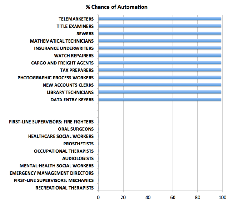
The Atlantic Monthly article cited above has an interesting graphic –

jobsautomationSo at the top of this chart are the jobs which are at 100 percent risk of being automated, while at the bottom are jobs which probably will never be automated (although I do think counseling can be done to a certain degree by AI applications).

The Final Frontier

This blog focuses on many of the relevant techniques in machine learning – basically unsupervised learning of patterns – which in the future will change everything.

Driverless cars are the wow example, of course.

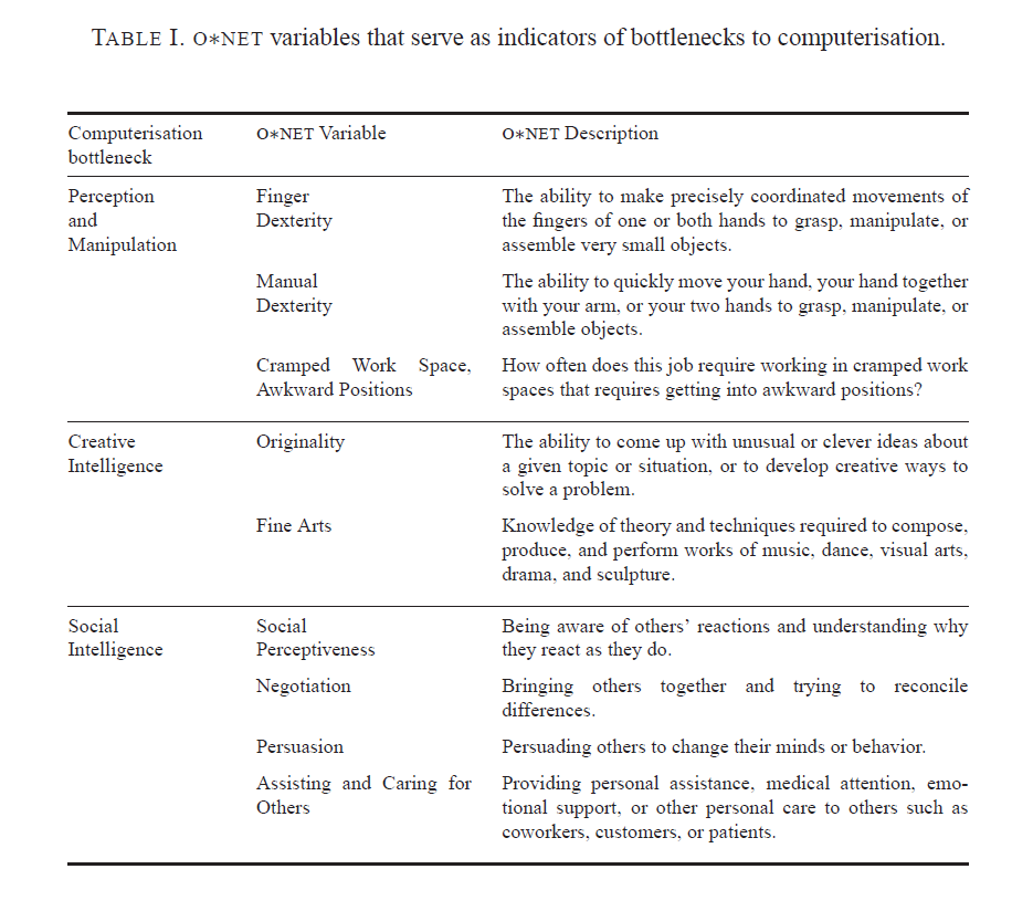
Bottlenecks to moving further up the curve of computerization are highlighted in the following table from the Oxford U report.

ONETvars

As far as dexterity and flexibility goes, Baxter shows great promise, as the following YouTube from his innovators illustrates.

There also are some wonderful examples of apparent creativity by computers or automatic systems, which I plan to detail in a future post.

Frey and Osborn, reflecting on their research in a 2014 discussion, conclude

So, if a computer can drive better than you, respond to requests as well as you and track down information better than you, what tasks will be left for labour? Our research suggests that human social intelligence and creativity are the domains were labour will still have a comparative advantage. Not least, because these are domains where computers complement our abilities rather than substitute for them. This is because creativity and social intelligence is embedded in human values, meaning that computers would not only have to become better, but also increasingly human, to substitute for labour performing such work.

Our findings thus imply that as technology races ahead, low-skill workers will need to reallocate to tasks that are non-susceptible to computerisation – i.e., tasks requiring creative and social intelligence. For workers to win the race, however, they will have to acquire creative and social skills. Development strategies thus ought to leverage the complementarity between computer capital and creativity by helping workers transition into new work, involving working with computers and creative and social ways.

Specifically, we recommend investing in transferable computer-related skills that are not particular to specific businesses or industries. Examples of such skills are computer programming and statistical modeling. These skills are used in a wide range of industries and occupations, spanning from the financial sector, to business services and ICT.

Implications For Business Forecasting

People specializing in forecasting for enterprise level business have some responsibility to “get ahead of the curve” – conceptually, at least.

Not everybody feels comfortable doing this, I realize.

However, I’m coming to the realization that these discussions of how many jobs are susceptible to “automation” or whatever you want to call it (not to mention jobs at risk for “offshoring”) – these discussions are really kind of the canary in the coal mine.

Something is definitely going on here.

But what are the metrics? Can you backdate the analysis Frey and Osborne offer, for example, to account for the coupling of productivity growth and slower employment gains since the last recession?

Getting a handle on this dynamic in the US, Europe, and even China has huge implications for marketing, and, indeed, social control.

The Tibshirani’s – Statistics and Machine Learning Superstars

As regular readers of this blog know, I’ve migrated to a weekly (or potentially longer) topic focus, and this week’s topic is variable selection.

And the next planned post in the series will compare and contrast ridge regression and the LASSO (least absolute shrinkage and selection operator). There also are some new results for the LASSO. But all this takes time and is always better when actual computations can be accomplished to demonstrate points.

But in researching this, I’ve come to a deeper appreciation of the Tibshiranis.

Robert Tibshirani was an early exponent of the LASSO and has probably, as much as anyone, helped integrate the LASSO into standard statistical procedures.

Here’s his picture from Wikipedia.

RobertTib2

You might ask why put his picuture up, and my answer is that Professor Robert Tibshirani (Stanford) has a son Ryan Tibshirani, whose picture is just below.

Ryan Tibsharani has a great Data Mining course online from Carnegie Mellon, where he is an Assistant Professor.

RyanTib

Professor Ryan Tibshirani’s Spring 2013 a Data Mining course can be found at http://www.stat.cmu.edu/~ryantibs/datamining/

Reviewing Ryan Tibsharani’s slides is very helpful in getting insight into topics like cross validation, ridge regression and the LASSO.

And let us not forget Professor Ryan Tibshirani is author of essential reading about how to pick your target in darts, based on your skill level (hint – don’t go for the triple-20 unless you are good).

Free Books on Machine Learning and Statistics

Robert Tibshirani et al’s text – Elements of Statistical Learning is now in the 10th version and is available online free here.

But the simpler An Introduction to Statistical Leaning is also available for an online download of a PDF file here. This is the corrected 4th printing. The book, which I have been reading today, is really dynamite – an outstanding example of scientific exposition and explanation.

These guys and their collaborators are truly gifted teachers. They create windows into new mathematical and statistical worlds, as it were.

Medical/Health Predictive Analytics – Logistic Regression

The case for assessing health risk with logistic regression is made by authors of a 2009 study, which is also a sort of model example for Big Data in diagnostic medicine.

As the variables that help predict breast cancer increase in number, physicians must rely on subjective impressions based on their experience to make decisions. Using a quantitative modeling technique such as logistic regression to predict the risk of breast cancer may help radiologists manage the large amount of information available, make better decisions, detect more cancers at early stages, and reduce unnecessary biopsies

This study – A Logistic Regression Model Based on the National Mammography Database Format to Aid Breast Cancer Diagnosis  – pulled together 62,219 consecutive mammography records from 48,744 studies in 18,270 patients reported using the Breast Imaging Reporting and Data System (BI-RADS) lexicon and the National Mammography Database format between April 5, 1999 and February 9, 2004.

The combination of medical judgment and an algorithmic diagnostic tool based on extensive medical records is, in the best sense, the future of medical diagnosis and treatment.

And logistic regression has one big thing going for it – a lot of logistic regressions have been performed to identify risk factors for various diseases or for mortality from a particular ailment.

A logistic regression, of course, maps a zero/one or categorical variable onto a set of explanatory variables.

This is not to say that there are not going to be speedbumps along the way. Interestingly, these are data science speedbumps, what some would call statistical modeling issues.

Picking the Right Variables, Validating the Logistic Regression

The problems of picking the correct explanatory variables for a logistic regression and model validation are linked.

The problem of picking the right predictors for a logistic regression is parallel to the problem of picking regressors in, say, an ordinary least squares (OLS) regression with one or two complications. You need to try various specifications (sets of explanatory variables) and utilize a raft of diagnostics to evaluate the different models. Cross-validation, utilized in the breast cancer research mentioned above, is probably better than in-sample tests. And, in addition, you need to be wary of some of the weird features of logistic regression.

A survey of medical research from a few years back highlights the fact that a lot of studies shortcut some of the essential steps in validation.

A Short Primer on Logistic Regression

I want to say a few words about how the odds-ratio is the key to what logistic regression is all about.

Logistic regression, for example, does not “map” a predictive relationship onto a discrete, categorical index, typically a binary, zero/one variable, in the same way ordinary least squares (OLS) regression maps a predictive relationship onto dependent variables. In fact, one of the first things one tends to read, when you broach the subject of logistic regression, is that, if you try to “map” a binary, 0/1 variable onto a linear relationship β01x12x2 with OLS regression, you are going to come up against the problem that the predictive relationship will almost always “predict” outside the [0,1] interval.

Instead, in logistic regression we have a kind of background relationship which relates an odds-ratio to a linear predictive relationship, as in,

ln(p/(1-p)) = β01x12x2

Here p is a probability or proportion and the xi are explanatory variables. The function ln() is the natural logarithm to the base e (a transcendental number), rather than the logarithm to the base 10.

The parameters of this logistic model are β0, β1, and β2.

This odds ratio is really primary and from the logarithm of the odds ratio we can derive the underlying probability p. This probability p, in turn, governs the mix of values of an indicator variable Z which can be either zero or 1, in the standard case (there being a generalization to multiple discrete categories, too).

Thus, the index variable Z can encapsulate discrete conditions such as hospital admissions, having a heart attack, or dying – generally, occurrences and non-occurrences of something.

Chinesemathteacher

It’s exactly analogous to flipping coins, say, 100 times. There is a probability of getting a heads on a flip, usually 0.50. The distribution of the number of heads in 100 flips is a binomial, where the probability of getting say 60 heads and 40 tails is the combination of 100 things taken 60 at a time, multiplied into (0.5)60*(0.5)40. The combination of 100 things taken 60 at a time equals 60!/(60!40!) where the exclamation mark indicates “factorial.”

Similarly, the probability of getting 60 occurrences of the index Z=1 in a sample of 100 observations is (p)60*(1-p)40multiplied by 60!/(60!40!).

The parameters βi in a logistic regression are estimated by means of maximum likelihood (ML).  Among other things, this can mean the optimal estimates of the beta parameters – the parameter values which maximize the likelihood function – must be estimated by numerical analysis, there being no closed form solutions for the optimal values of β0, β1, and β2.

In addition, interpretation of the results is intricate, there being no real consensus on the best metrics to test or validate models.

SAS and SPSS as well as software packages with smaller market shares of the predictive analytics space, offer algorithms, whereby you can plug in data and pull out parameter estimates, along with suggested metrics for statistical significance and goodness of fit.

There also are logistic regression packages in R.

But you can do a logistic regression, if the data are not extensive, with an Excel spreadsheet.

This can be instructive, since, if you set it up from the standpoint of the odds-ratio, you can see that only certain data configurations are suitable. These configurations – I refer to the values which the explanatory variables xi can take, as well as the associated values of the βi – must be capable of being generated by the underlying probability model. Some data configurations are virtually impossible, while others are inconsistent.

This is a point I find lacking in discussions about logistic regression, which tend to note simply that sometimes the maximum likelihood techniques do not converge, but explode to infinity, etc.

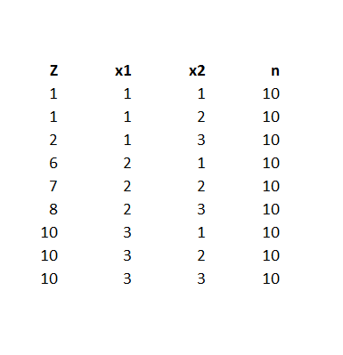
Here is a spreadsheet example, where the predicting equation has three parameters and I determine the underlying predictor equation to be,

ln(p/(1-p))=-6+3x1+.05x2

and we have the data-
logisticregmodel

Notice the explanatory variables x1 and x2 also are categorical, or at least, discrete, and I have organized the data into bins, based on the possible combinations of the values of the explanatory variables – where the number of cases in each of these combinations or populations is given to equal 10 cases. A similar setup can be created if the explanatory variables are continuous, by partitioning their ranges and sorting out the combination of ranges in however many explanatory variables there are, associating the sum of occurrences associated with these combinations. The purpose of looking at the data this way, of course, is to make sense of an odds-ratio.

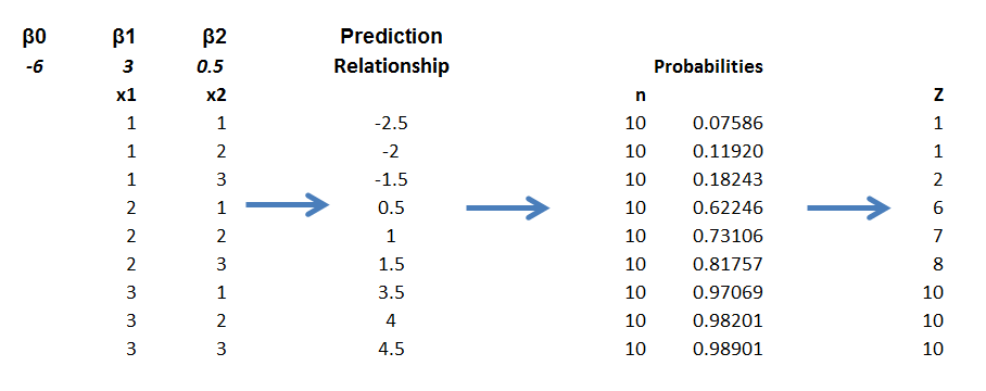
The predictor equation above in the odds ratio can be manipulated into a form which explicitly indicates the probability of occurrence of something or of Z=1. Thus,

p= eβ0+β1×1+β2×2/(1+ eβ0+β1×1+β2×2)

where this transformation takes advantage of the principle that elny = y.

So with this equation for p, I can calculate the probabilities associated with each of the combinations in the data rows of the spreadsheet. Then, given the probability of that configuration, I calculate the expected value of Z=1 by the formula 10p. Thus, the mean of a binomial variable with probability p is np, where n is the number of trials. This sequence is illustrated below (click to enlarge).
sequence

Picking the “success rates” for each of the combinations to equal the expected value of the occurrences, given 10 “trials,” produces a highly consistent set of data.

Along these lines, the most valuable source I have discovered for ML with logistic regression is a paper by Scott
Czepiel – Maximum Likelihood Estimation of Logistic Regression Models: Theory and Implementation
.

I can readily implement Czepiel’s log likelihood function in his Equation (9) with an Excel spreadsheet and Solver.

It’s also possible to see what can go wrong with this setup.

For example, the standard deviation of a binomial process with probability p and n trials is np(1-p). If we then simulate the possible “occurrences” for each of the nine combinations, some will be closer to the estimate of np used in the above spreadsheet, others will be more distant. Peforming such simulations, however, highlights that some numbers of occurrences for some combinations will simply never happen, or are well nigh impossible, based on the laws of chance.

Of course, this depends on the values of the parameters selected, too – but it’s easy to see that, whatever values selected for the parameters, some low probability combinations will be highly unlikely to produce a high number for successes. This results in a nonconvergent ML process, so some parameters simply may not be able to be estimated.

This means basically that logistic regression is less flexible in some sense than OLS regression, where it is almost always possible to find values for the parameters which map onto the dependent variable.

What This Means

Logistic regression, thus, is not the exact analogue of OLS regression, but has nuances of its own. This has not prohibited its wide application in medical risk assessment (and I am looking for a survey article which really shows the extent of its application across different medical fields).

There also are more and more reports of the successful integration of medical diagnostic systems, based in some way on logistic regression analysis, in informing medical practices.

But the march of data science is relentless. Just when doctors got a handle on logistic regression, we have a raft of new techniques, such as random forests and splines.

Header image courtesy of: National Kidney & Urologic Diseases Information Clearinghouse (NKUDIC)

Predicting the Market Over Short Time Horizons

Google “average time a stock is held.” You will come up with figures that typically run around 20 seconds. High frequency trades (HFT) dominate trading volume on the US exchanges.

All of which suggests the focus on the predictability of stock returns needs to position more on intervals lasting seconds or minutes, rather than daily, monthly, or longer trading periods.

So, it’s logical that Michael Rechenthin, a newly minted Iowa Ph.D., and Nick Street, a Professor of Management, are getting media face time from research which purportedly demonstrates the existence of predictable short-term trends in the market (see Using conditional probability to identify trends in intra-day high-frequency equity pricing).

Here’s the abstract –

By examining the conditional probabilities of price movements in a popular US stock over different high-frequency intra-day timespans, varying levels of trend predictability are identified. This study demonstrates the existence of predictable short-term trends in the market; understanding the probability of price movement can be useful to high-frequency traders. Price movement was examined in trade-by-trade (tick) data along with temporal timespans between 1 s to 30 min for 52 one-week periods for one highly-traded stock. We hypothesize that much of the initial predictability of trade-by-trade (tick) data is due to traditional market dynamics, or the bouncing of the price between the stock’s bid and ask. Only after timespans of between 5 to 10 s does this cease to explain the predictability; after this timespan, two consecutive movements in the same direction occur with higher probability than that of movements in the opposite direction. This pattern holds up to a one-minute interval, after which the strength of the pattern weakens.

The study examined price movements of the exchange traded fund SPY, during 2005, finding that

.. price movements can be predicted with a better than 50-50 accuracy for anywhere up to one minute after the stock leaves the confines of its bid-ask spread. Probabilities continue to be significant until about five minutes after it leaves the spread. By 30 minutes, the predictability window has closed.

Of course, the challenges of generalization in this world of seconds and minutes is tremendous. Perhaps, for example, the patterns the authors identify are confined to the year of the study. Without any theoretical basis, brute force generalization means riffling through additional years of 31.5 million seconds each.

Then, there are the milliseconds, and the recent blockbuster written by Michael Lewis – Flash Boys: A Wall Street Revolt.

I’m on track for reading this book for a bookclub to which I belong.

As I understand it, Lewis, who is one of my favorite financial writers, has uncovered a story whereby high frequency traders, operating with optical fiber connections to the New York Stock Exchange, sometimes being geographically as proximate as possible, can exploit more conventional trading – basically buying a stock after you have put in a buy order, but before your transaction closes, thus raising your price if you made a market order.

MLewis

The LA Times  has a nice review of the book and ran the above photo of Lewis.

Forecasting Housing Markets – 3

Maybe I jumped to conclusions yesterday. Maybe, in fact, a retrospective analysis of the collapse in US housing prices in the recent 2008-2010 recession has been accomplished – but by major metropolitan area.

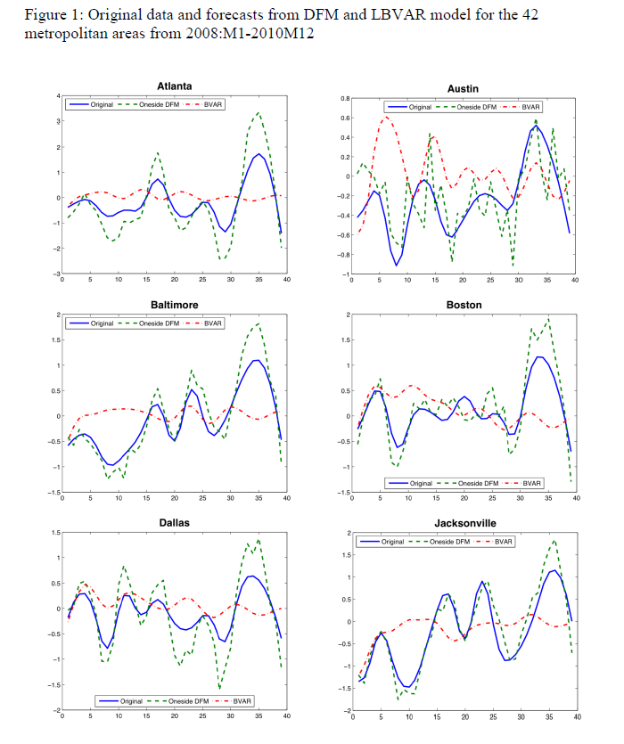
The Yarui Li and David Leatham paper Forecasting Housing Prices: Dynamic Factor Model versus LBVAR Model focuses on out-of-sample forecasts for house price indices for 42 metropolitan areas. Forecast models are built with data from 1980:01 to 2007:12. These models – dynamic factor and Large-scale Bayesian Vector Autoregressive (LBVAR) models – are used to generate forecasts of the one- to twelve- months ahead price growth 2008:01 to 2010:12.

Judging from the graphics and other information, the dynamic factor model (DFM) produces impressive results.

For example, here are out-of-sample forecasts of the monthly growth of housing prices (click to enlarge).

DFMhousing

The house price indices for the 42 metropolitan areas are from the Office of Federal Housing Enterprise Oversight (OFEO). The data for macroeconomic indicators in the dynamic factor and VAR models are from the DRI/McGraw Hill Basic Economics Database provided by IHS Global Insight.

I have seen forecasting models using Internet search activity which purportedly capture turning points in housing price series, but this is something different.

The claim here is that calculating dynamic or generalized principal components of some 141 macroeconomic time series can lead to forecasting models which accurately capture fluctuations in cumulative growth rates of metropolitan house price indices over a forecasting horizon of up to 12 months.

That’s pretty startling, and I for one would like to see further output of such models by city.

But where is the publication of the final paper? The PDF file linked above was presented at the Agricultural & Applied Economics Association’s 2011 Annual Meeting in Pittsburgh, Pennsylvania, July, 2011. A search under both authors does not turn up a final publication in a refereed journal, but does indicate there is great interest in this research. The presentation paper thus is available from quite a number of different sources which obligingly archive it.

Yarui

Currently, the lead author, Yarui Li, Is a Decision Tech Analyst at JPMorgan Chase, according to LinkedIn, having received her PhD from Texas A&M University in 2013. The second author is Professor at Texas A&M, most recently publishing on VAR models applied to business failure in the US.

Dynamic Principal Components

It may be that dynamic principal components are the new ingredient accounting for an uncanny capability to identify turning points in these dynamic factor model forecasts.

The key research is associated with Forni and others, who originally documented dynamic factor models in the Review of Economics and Statistics in 2000. Subsequently, there have been two further publications by Forni on this topic:

Do financial variables help forecasting inflation and real activity in the euro area?

The Generalized Dynamic Factor Model, One Sided Estimation and Forecasting

Forni and associates present this method of dynamic prinicipal componets as an alternative to the Stock and Watson factor models based on many predictors – an alternative with superior forecasting performance.

Run-of-the-mill standard principal components are, according to Li and Leatham, based on contemporaneous covariances only. So they fail to exploit the potentially crucial information contained in the leading-lagging relations between the elements of the panel.

By contrast, the Forni dynamic component approach is used in this housing price study to

obtain estimates of common and idiosyncratic variance-covariance matrices at all leads and lags as inverse Fourier transforms of the corresponding estimated spectral density matrices, and thus overcome(s)[ing] the limitation of static PCA.

There is no question but that any further discussion of this technique must go into high mathematical dudgeon, so I leave that to another time, when I have had an opportunity to make computations of my own.

However, I will say that my explorations with forecasting principal components last year have led to me to wonder whether, in fact, it may be possible to pull out some turning points from factor models based on large panels of macroeconomic data.

Flu Forecasting and Google – An Emerging Big Data Controversy

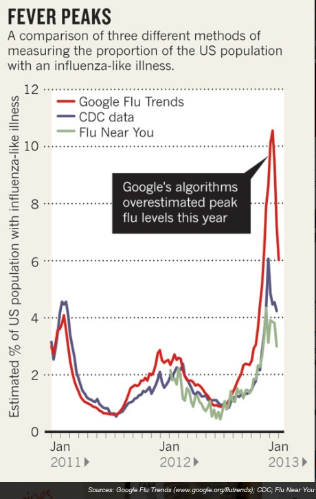
It started innocently enough, when an article in the scientific journal Nature caught my attention – When Google got flu wrong. This highlights big errors in Google flu trends in the 2012-2013 flu season.

flutrends

Then digging into the backstory, I’m intrigued to find real controversy bubbling below the surface. Phrases like “big data hubris” are being thrown around, and there are insinuations Google is fudging model outcomes, at least in backtests. Beyond that, there are substantial statistical criticisms of the Google flu trends model – relating to autocorrelation and seasonality of residuals.

I’m using this post to keep track of some of the key documents and developments.

Background on Google Flu Trends

Google flu trends, launched in 2008, targets public health officials, as well as the general public.

Cutting lead-time on flu forecasts can support timely stocking and distribution of vaccines, as well as encourage health practices during critical flue months.

What’s the modeling approach?

There seem to be two official Google-sponsored reports on the underlying prediction model.

Detecting influenza epidemics using search engine query data appears in Nature in early 2009, and describes a logistic regression model estimating the probability that a random physician visit in a particular region is related to an influenza-like illness (ILI). This approach is geared to historical logs of online web search queries submitted between 2003 and 2008, and publicly available data series from the CDC’s US Influenza Sentinel Provider Surveillance Network (http://www.cdc.gov/flu/weekly).

The second Google report – Google Disease Trends: An Update – came out recently, in response to our algorithm overestimating influenza-like illness (ILI) and the 2013 Nature article. It mentions in passing corrections discussed in a 2011 research study, but focuses on explaining the over-estimate in peak doctor visits during the 2012-2013 flu season.

The current model, while a well performing predictor in previous years, did not do very well in the 2012-2013 flu season and significantly deviated from the source of truth, predicting substantially higher incidence of ILI than the CDC actually found in their surveys. It became clear that our algorithm was susceptible to bias in situations where searches for flu-related terms on Google.com were uncharacteristically high within a short time period. We hypothesized that concerned people were reacting to heightened media coverage, which in turn created unexpected spikes in the query volume. This assumption led to a deep investigation into the algorithm that looked for ways to insulate the model from this type of media influence

The antidote – “spike detectors” and more frequent updating.

The Google Flu Trends Still Appears Sick Report

A just-published critique –Google Flu Trends Still Appears Sick – available as a PDF download from a site at Harvard University – provides an in-depth review of the errors and failings of Google foray into predictive analytics. This latest critique of Google flu trends even raises the issue of “transparency” of the modeling approach and seems to insinuate less than impeccable honesty at Google with respect to model performance and model details.

This white paper follows the March 2014 publication of The Parable of Google Flu: Traps in Big Data Analysis in Science magazine. The Science magazine article identifies substantive statistical problems with the Google flu trends modeling, such as the fact that,

..the overestimation problem in GFT was also present in the 2011‐2012 flu season (2). The report also found strong evidence of autocorrelation and seasonality in the GFT errors, and presented evidence that the issues were likely, at least in part, due to modifications made by Google’s search algorithm and the decision by GFT engineers not to use previous CDC reports or seasonality estimates in their models – what the article labeled “algorithm dynamics” and “big data hubris” respectively.

Google Flu Trends Still Appears Sick follows up on the very recent science article, pointing out that the 2013-2014 flu season also shows fairly large errors, and asking –

So have these changes corrected the problem? While it is impossible to say for sure based on one subsequent season, the evidence so far does not look promising. First, the problems identified with replication in GFT appear to, if anything, have gotten worse. Second, the evidence that the problems in 2012‐2013 were due to media coverage is tenuous. While GFT engineers have shown that there was a spike in coverage during the 2012‐2013 season, it seems unlikely that this spike was larger than during the 2005‐2006 A/H5N1 (“bird flu”) outbreak and the 2009 A/H1N1 (“swine flu”) pandemic. Moreover, it does not explain why the proportional errors were so large in the 2011‐2012 season. Finally, while the changes made have dampened the propensity for overestimation by GFT, they have not eliminated the autocorrelation and seasonality problems in the data.

The white paper authors also highlight continuing concerns with Google’s transparency.

One of our main concerns about GFT is the degree to which the estimates are a product of a highly nontransparent process… GFT has not been very forthcoming with this information in the past, going so far as to release misleading example search terms in previous publications (2, 3, 8). These transparency problems have, if anything, become worse. While the data on the intensity of media coverage of flu outbreaks does not involve privacy concerns, GFT has not released this data nor have they provided an explanation of how the information was collected and utilized. This information is critically important for future uses of GFT. Scholars and practitioners in public health will need to be aware of where the information on media coverage comes from and have at least a general idea of how it is applied in order to understand how to interpret GFT estimates the next time there is a season with both high flu prevalence and high media coverage.

They conclude by stating that GFT is still ignoring data that could help it avoid future problems.

Finally, to really muddy the waters Columbia University medical researcher Jeffrey Shaman recently announced First Real-Time Flu Forecast Successful. Shaman’s model apparently keys off Google flu trends.

What Does This Mean?

I think the Google flu trends controversy is important for several reasons.

First, predictive models drawing on internet search activity and coordinated with real-time clinical information are an ambitious and potentially valuable undertaking, especially if they can provide quicker feedback on prospective ILI in specific metropolitan areas. And the Google teams involved in developing and supporting Google flu trends have been somewhat forthcoming in presenting their modeling approach and acknowledging problems that have developed.

“Somewhat” but not fully forthcoming – and that seems to be the problem. Unlike research authored by academicians or the usual scientific groups, the authors of the two main Google reports mentioned above remain difficult to reach directly, apparently. So question linger and critics start to get impatient.

And it appears that there are some standard statistical issues with the Google flu forecasts, such as autocorrelation and seasonality in residuals that remain uncorrected.

I guess I am not completely surprised, since the Google team may have come from the data mining or machine learning community, and not be sufficiently indoctrinated in the “old ways” of developing statistical models.

Craig Venter has been able to do science, and yet operate in private spaces, rather than in the government or nonprofit sector. Whether Google as a company will allow scientific protocols to be followed – as apparently clueless as these are to issues of profit or loss – remains to be seen. But if we are going to throw the concept of “data scientist” around, I guess we need to think through the whole package of stuff that goes with that.

Three Pass Regression Filter – New Data Reduction Method

Malcolm Gladwell’s 10,000 hour rule (for cognitive mastery) is sort of an inspiration for me. I picked forecasting as my field for “cognitive mastery,” as dubious as that might be. When I am directly engaged in an assignment, at some point or other, I feel the need for immersion in the data and in estimations of all types. This blog, on the other hand, represents an effort to survey and, to some extent, get control of new “tools” – at least in a first pass. Then, when I have problems at hand, I can try some of these new techniques.

Ok, so these remarks preface what you might call the humility of my approach to new methods currently being innovated. I am not putting myself on a level with the innovators, for example. At the same time, it’s important to retain perspective and not drop a critical stance.

The Working Paper and Article in the Journal of Finance

Probably one of the most widely-cited recent working papers is Kelly and Pruitt’s three pass regression filter (3PRF). The authors, shown above, are with the University of Chicago, Booth School of Business and the Federal Reserve Board of Governors, respectively, and judging from the extensive revisions to the 2011 version, they had a bit of trouble getting this one out of the skunk works.

Recently, however, Kelly and Pruit published an important article in the prestigious Journal of Finance called Market Expectations in the Cross-Section of Present Values. This article applies a version of the three pass regression filter to show that returns and cash flow growth for the aggregate U.S. stock market are highly and robustly predictable.

I learned of a published application of the 3PRF from Francis X. Dieblod’s blog, No Hesitations, where Diebold – one of the most published authorities on forecasting – writes

Recent interesting work, moreover, extends PLS in powerful ways, as with the Kelly-Pruitt three-pass regression filter and its amazing apparent success in predicting aggregate equity returns.

What is the 3PRF?

The working paper from the Booth School of Business cited at a couple of points above describes what might be cast as a generalization of partial least squares (PLS). Certainly, the focus in the 3PRF and PLS is on using latent variables to predict some target.

I’m not sure, though, whether 3PRF is, in fact, more of a heuristic, rather than an algorithm.

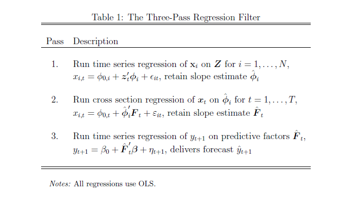
What I mean is that the three pass regression filter involves a procedure, described below.

(click to enlarge).

3PRFprocedure

Here’s the basic idea –

Suppose you have a large number of potential regressors xi ε X, i=1,..,N. In fact, it may be impossible to calculate an OLS regression, since N > T the number of observations or time periods.

Furthermore, you have proxies zj ε  Z, I = 1,..,L – where L is significantly less than the number of observations T. These proxies could be the first several principal components of the data matrix, or underlying drivers which theory proposes for the situation. The authors even suggest an automatic procedure for generating proxies in the paper.

And, finally, there is the target variable yt which is a column vector with T observations.

Latent factors in a matrix F drive both the proxies in Z and the predictors in X. Based on macroeconomic research into dynamic factors, there might be only a few of these latent factors – just as typically only a few principal components account for the bulk of variation in a data matrix.

Now here is a key point – as Kelly and Pruitt present the 3PRF, it is a leading indicator approach when applied to forecasting macroeconomic variables such as GDP, inflation, or the like. Thus, the time index for yt ranges from 2,3,…T+1, while the time indices of all X and Z variables and the factors range from 1,2,..T. This means really that all the x and z variables are potentially leading indicators, since they map conditions from an earlier time onto values of a target variable at a subsequent time.

What Table 1 above tells us to do is –

  1. Run an ordinary least square (OLS) regression of the xi      in X onto the zj in X, where T ranges from 1 to T and there are      N variables in X and L << T variables in Z. So, in the example      discussed below, we concoct a spreadsheet example with 3 variables in Z,      or three proxies, and 10 predictor variables xi in X (I could      have used 50, but I wanted to see whether the method worked with lower      dimensionality). The example assumes 40 periods, so t = 1,…,40. There will      be 40 different sets of coefficients of the zj as a result of      estimating these regressions with 40 matched constant terms.
  2. OK, then we take this stack of estimates of      coefficients of the zj and their associated constants and map      them onto the cross sectional slices of X for t = 1,..,T. This means that,      at each period t, the values of the cross-section. xi,t, are      taken as the dependent variable, and the independent variables are the 40      sets of coefficients (plus constant) estimated in the previous step for      period t become the predictors.
  3. Finally, we extract the estimate of the factor loadings      which results, and use these in a regression with target variable as the      dependent variable.

This is tricky, and I have questions about the symbolism in Kelly and Pruitt’s papers, but the procedure they describe does work. There is some Matlab code here alongside the reference to this paper in Professor Kelly’s research.

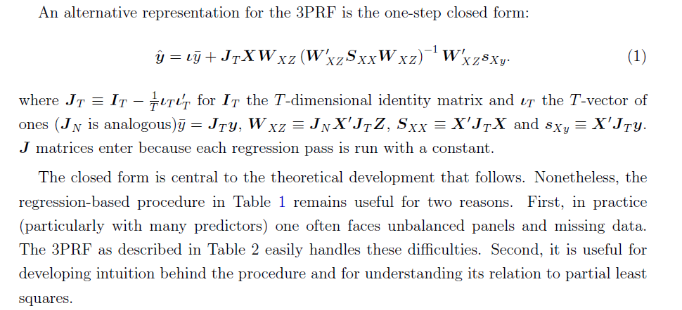
At the same time, all this can be short-circuited (if you have adequate data without a lot of missing values, apparently) by a single humungous formula –

3PRFformula

Here, the source is the 2012 paper.

Spreadsheet Implementation

Spreadsheets help me understand the structure of the underlying data and the order of calculation, even if, for the most part, I work with toy examples.

So recently, I’ve been working through the 3PRF with a small spreadsheet.

Generating the factors:I generated the factors as two columns of random variables (=rand()) in Excel. I gave the factors different magnitudes by multiplying by different constants.

Generating the proxies Z and predictors X. Kelly and Pruitt call for the predictors to be variance standardized, so I generated 40 observations on ten sets of xi by selecting ten different coefficients to multiply into the two factors, and in each case I added a normal error term with mean zero and standard deviation 1. In Excel, this is the formula =norminv(rand(),0,1).

Basically, I did the same drill for the three zj — I created 40 observations for z1, z2, and z3 by multiplying three different sets of coefficients into the two factors and added a normal error term with zero mean and variance equal to 1.

Then, finally, I created yt by multiplying randomly selected coefficients times the factors.

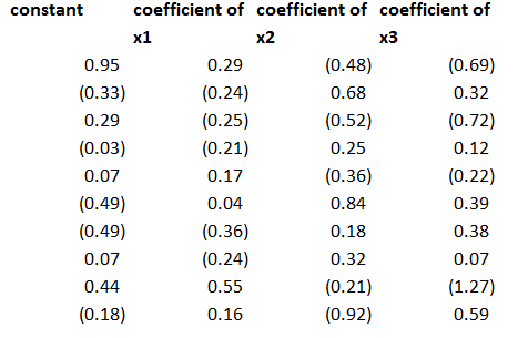
After generating the data, the first pass regression is easy. You just develop a regression with each predictor xi as the dependent variable and the three proxies as the independent variables, case-by-case, across the time series for each. This gives you a bunch of regression coefficients which, in turn, become the explanatory variables in the cross-sectional regressions of the second step.

The regression coefficients I calculated for the three proxies, including a constant term, were as follows – where the 1st row indicates the regression for x1 and so forth.

coeff

This second step is a little tricky, but you just take all the values of the predictor variables for a particular period and designate these as the dependent variables, with the constant and coefficients estimated in the previous step as the independent variables. Note, the number of predictors pairs up exactly with the number of rows in the above coefficient matrix.

This then gives you the factor loadings for the third step, where you can actually predict yt (really yt+1 in the 3PRF setup). The only wrinkle is you don’t use the constant terms estimated in the second step, on the grounds that these reflect “idiosyncratic” effects, according to the 2011 revision of the paper.

Note the authors describe this as a time series approach, but do not indicate how to get around some of the classic pitfalls of regression in a time series context. Obviously, first differencing might be necessary for nonstationary time series like GDP, and other data massaging might be in order.

Bottom line – this worked well in my first implementation.

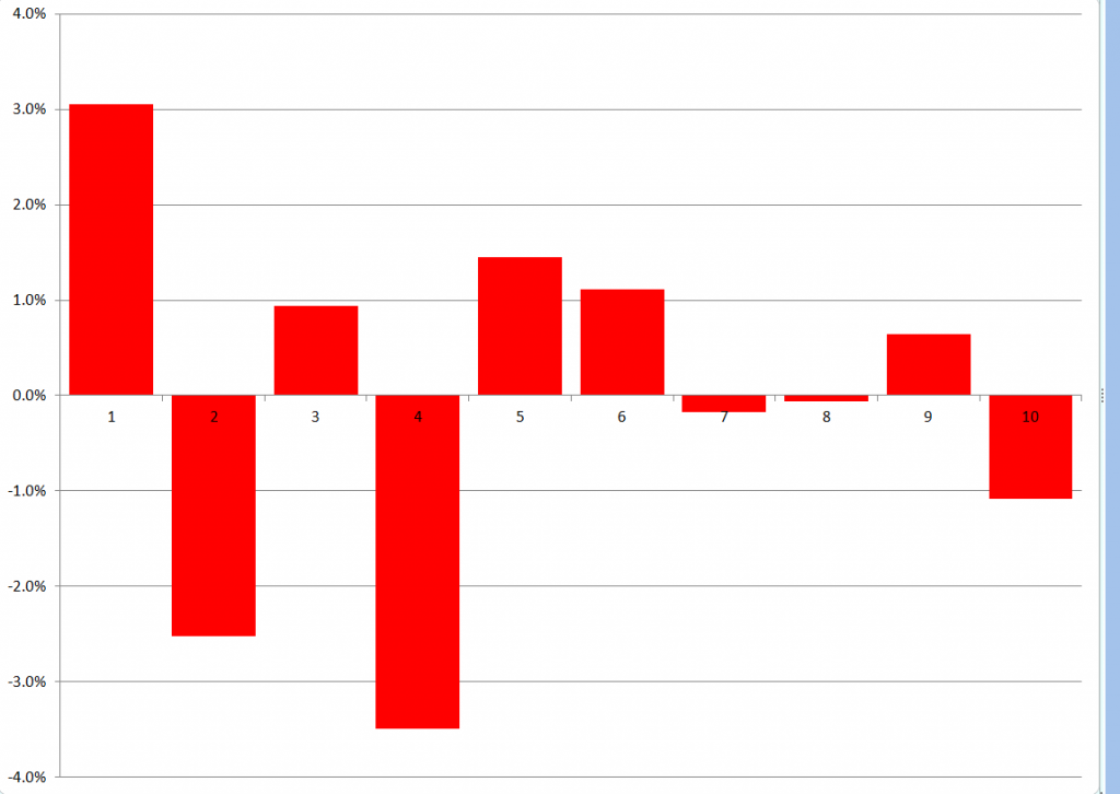
To forecast, I just used the last regression for yt+1 and then added ten more cases, calculating new values for the target variable with the new values of the factors. I used the new values of the predictors to update the second step estimate of factor loadings, and applied the last third pass regression to these values.

Here are the forecast errors for these ten out-of-sample cases.

3PRFforecasterror

Not bad for a first implementation.

 Why Is Three Pass Regression Important?

3PRF is a fairly “clean” solution to an important problem, relating to the issue of “many predictors” in macroeconomics and other business research.

Noting that if the predictors number near or more than the number of observations, the standard ordinary least squares (OLS) forecaster is known to be poorly behaved or nonexistent, the authors write,

How, then, does one effectively use vast predictive information? A solution well known in the economics literature views the data as generated from a model in which latent factors drive the systematic variation of both the forecast target, y, and the matrix of predictors, X. In this setting, the best prediction of y is infeasible since the factors are unobserved. As a result, a factor estimation step is required. The literature’s benchmark method extracts factors that are significant drivers of variation in X and then uses these to forecast y. Our procedure springs from the idea that the factors that are relevant to y may be a strict subset of all the factors driving X. Our method, called the three-pass regression filter (3PRF), selectively identifies only the subset of factors that influence the forecast target while discarding factors that are irrelevant for the target but that may be pervasive among predictors. The 3PRF has the advantage of being expressed in closed form and virtually instantaneous to compute.

So, there are several advantages, such as (1) the solution can be expressed in closed form (in fact as one complicated but easily computable matrix expression), and (2) there is no need to employ maximum likelihood estimation.

Furthermore, 3PRF may outperform other approaches, such as principal components regression or partial least squares.

The paper illustrates the forecasting performance of 3PRF with real-world examples (as well as simulations). The first relates to forecasts of macroeconomic variables using data such as from the Mark Watson database mentioned previously in this blog. The second application relates to predicting asset prices, based on a factor model that ties individual assets’ price-dividend ratios to aggregate stock market fluctuations in order to uncover investors’ discount rates and dividend growth expectations.