Category Archives: financial forecasts

Investment and Other Bank Macro Forecasts and Outlooks – 1

In yesterday’s post, I detailed the IMF World Economic Outlook revision for October 2014, recent OECD macroeconomic projections,  and latest from the Survey of Professional Forecasters.

All these are publically available, quite comprehensive forecasts, sort of standards in the field.

But there also are a range of private forecasts, and I want to focus on investment and other bank forecasts for the next few posts – touching on Goldman Sachs and JP Morgan today.

Goldman Sachs

Goldman Sachs – video presentations on global economic outlook with additional videos for the US, Europe, and major global regions. December 2013

Goldman Sachs, Economic Outlook for the United States, June 2014, Jan Hatzius

Goldman Sachs Asset Management, FISG Quarterly Outlook Q4 2014, (click on the right of the page for Full Document). This is the most up-to-date forecast/commentary I am able to find, and has a couple of relevant points.

One concerns the policy divergence at the central bank level. This is even more true now than when the report was released (probably in October), since the Bank of Japan is plunging into new, aggressive quantitative easing (QE), while the US Fed has ended its QE program, for the time being at least.

The other point concerns the European economy.

Among our economic forecasts, our negative outlook on the Eurozone represents the biggest departure from consensus. We believe policymakers will struggle to correct the trend of poor growth and disinflation. Optimism about the peripheries has faded, and the Eurozone’s powerhouse economy, Germany, has slowed amid weak global demand. Once again the Eurozone’s political divisions and fiscal constraints leave the ECB as the only authority able to respond unilaterally to the threat of a sharper downturn, though hopes of fiscal action are mounting.

Some signs of a sustainable Eurozone recovery have not held up to closer inspection. The peripheries have made substantial progress on austerity and structural reforms, but efforts appear to have stalled, and Spain has probably reaped the most it can from its adjustment for now. Italy’s policy paralysis and relapse into recession is disappointing given this year’s changing of the political guard, which saw Silvio Berlusconi’s exit and Prime Minister Matteo Renzi’s election on a heavily reformist platform. Renzi has shifted gears from political reform to labor reform, which could get under way in early 2015. But Italy’s high debt stock makes it particularly vulnerable to a market backlash, and we are watching for signs of investor pullback that could drive sovereign yields higher.

JP Morgan

JP Morgan has a 2014 Economic Outlook in a special issue of their Thought magazine. This is definitely dated, but there is a weekly Economic Update in a kind of scorecard format (up/down/nochange) from their Asset Management Group.

I’ve got to say, however, that one of the most exciting publications along these lines is their quarterly Guide to the Markets from JP Morgan Asset Management. Here are highlights from an interactive version of the 4Q Guide.

First, the scope of coverage is impressive, although, note this is more of an update of conditions, than a forecast. The reader supplies the forecasts, however, from these engaging slides.

contentsJPM

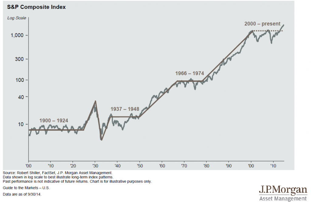
But this slide does not need to produce a forecast to make its point – which is maybe we are not in a stock market bubble but at the start of a long upward climb in the market. Optimism forever!

StockMarketSince 1900

There are plenty of slides that have moral to the story, such as this one on education and employment.

educationemp

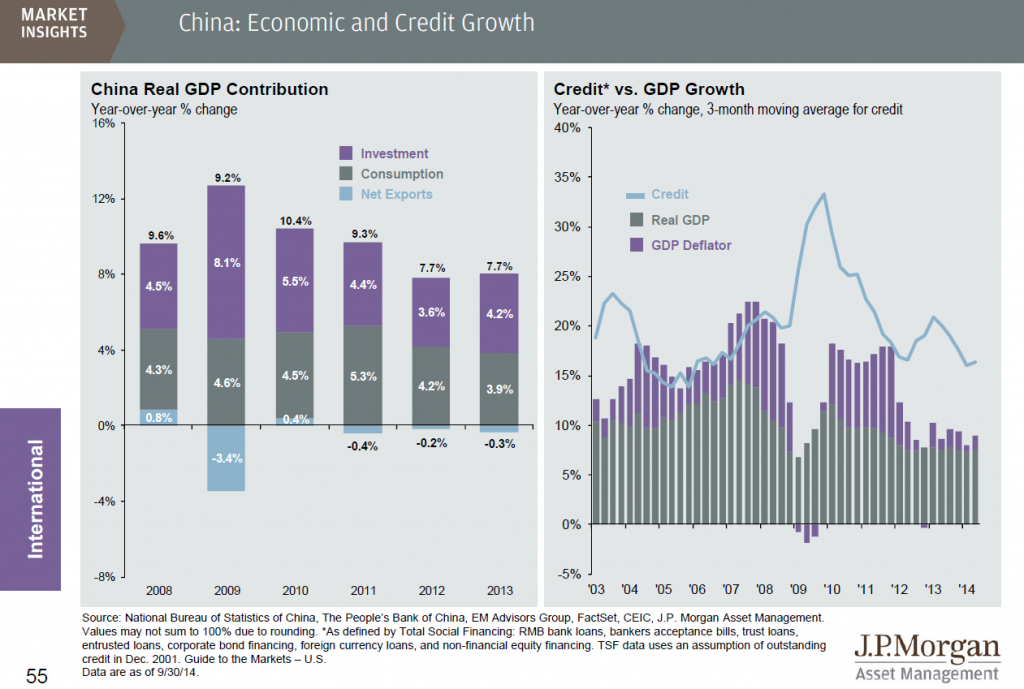
Then, this graphic on China is extremely revealing, and suggests a forward perspective.

chinastuff

I’m finding this excursion into bank forecasts productive and plan coming posts along these lines. I’d rather use the blog as a scratch-pad to share insights as I go along, than produce one humungous summary. So stay tuned.

Top photo courtesy of the University of Richmond

Something is Happening in Europe

Something is going on in Europe.

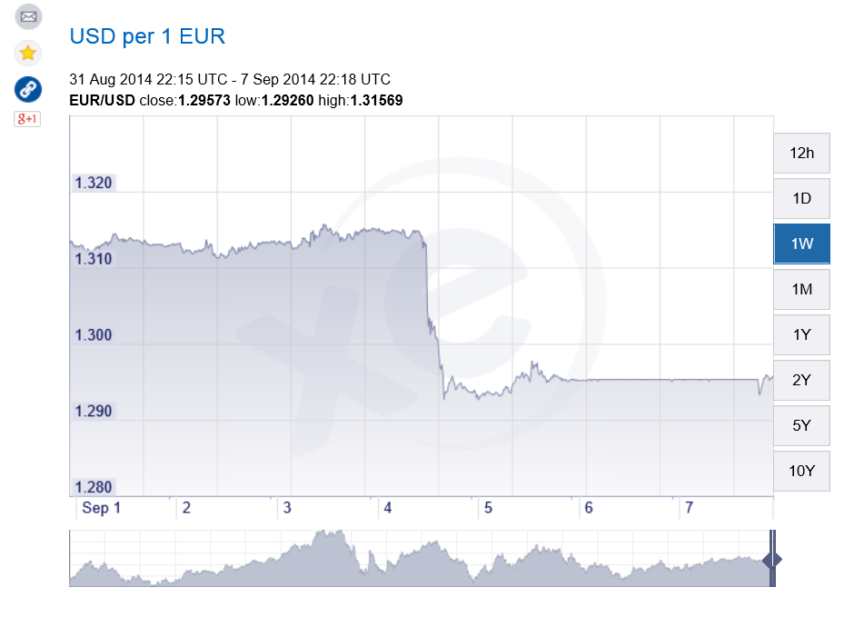
Take a look at this chart of the euro/dollar exchange rate, and how some event triggered a step down mid week of last week (from xe.com).

euroexchange

The event in question was a press conference by Mario Draghi (See the Wall Street Journal real time blog on this event at Mario Draghi Delivers Fresh ECB Plan — Recap).

The European Central Bank under Draghi is moving into exotic territory – trying negative interest rates on bank deposits and toying with variants of Quantitative Easing (QE) involving ABS – asset backed securities.

All because the basic numbers for major European economies, including notably Germany and France (as well as long-time problem countries such as Spain), are not good. Growth has stalled or is reversing, bank lending is falling, and deflation stalks the European markets.

Europe – which, of course, is sectored into the countries inside and outside the currency union, countries in the common market, and countries in none of the above – accounts for several hundred million persons and maybe 20-30 percent of global production.

So what happens there is significant.

Then there is the Ukraine crisis.

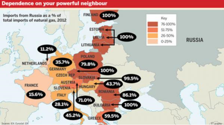
Zerohedge ran this graphic recently showing the dependence of European countries on gas from Russia.

eurdependence

The US-led program of imposing sanctions on Russia – key individuals, companies, banks perhaps – flies in the face of the physical dependence of Germany, for example, on Russian gas.

On the other hand, there is lots of history here on all sides, including, notably, the countries formerly in the USSR in eastern Europe, who no doubt fear the increasingly nationalistic or militant stance shown by Russia currently in, for example, re-acquiring Crimea.

As Chancellor Merkel has stressed, this is an area for diplomacy and negotiation – although there are other voices and forces ready to rush more weapons and even troops to the region of conflict.

Finally, as I have been stressing from time to time, there is an emerging demographic reality which many European nations have to confront.

Edward Hugh has several salient posts on possibly overlooked impacts of aging on the various macroeconomies involved.

There also is the vote on Scotland coming up in the United Kingdom (what we may, if the “yes” votes carry, need to start calling “the British Isles.”)

I’d like to keep current with the signals coming from Europe in a few blogs upcoming – to see, for example, whether swing events in the next six months to a year could originate there.

Forecasting Controversies – Impacts of QE

Where there is smoke, there is fire, and other similar adages are suggested by an arcane statistical controversy over quantitative easing (QE) by the US Federal Reserve Bank.

Some say this Fed policy, estimated to have involved $3.7 trillion dollars in asset purchases, has been a bust, a huge waste of money, a give-away program to speculators, but of no real consequence to Main Street.

Others credit QE as the main force behind lower long term interest rates, which have supported US housing markets.

Into the fray jump two elite econometricians – Johnathan Wright of Johns Hopkins and Christopher Neeley, Vice President of the St. Louis Federal Reserve Bank.

The controversy provides an ersatz primer in estimation and forecasting issues with VAR’s (vector autoregressions). I’m not going to draw out all the nuances, but highlight the main features of the argument.

The Effect of QE Announcements From the Fed Are Transitory – Lasting Maybe Two or Three Months

Basically, there is the VAR (vector autoregression) analysis of Johnathan Wright of Johns Hopkins Univeristy, which finds that  –

..stimulative monetary policy shocks lower Treasury and corporate bond yields, but the effects die o¤ fairly fast, with an estimated half-life of about two months.

This is in a paper What does Monetary Policy do to Long-Term Interest Rates at the Zero Lower Bound? made available in PDF format dated May 2012.

More specifically, Wright finds that

Over the period since November 2008, I estimate that monetary policy shocks have a significant effect on ten-year yields and long-maturity corporate bond yields that wear o¤ over the next few months. The effect on two-year Treasury yields is very small. The initial effect on corporate bond yields is a bit more than half as large as the effect on ten-year Treasury yields. This finding is important as it shows that the news about purchases of Treasury securities had effects that were not limited to the Treasury yield curve. That is, the monetary policy shocks not only impacted Treasury rates, but were also transmitted to private yields which have a more direct bearing on economic activity. There is slight evidence of a rotation in breakeven rates from Treasury Inflation Protected Securities (TIPS), with short-term breakevens rising and long-term forward breakevens falling.

Not So, Says A Federal Reserve Vice-President

Christopher Neeley at the St. Louis Federal Reserve argues Wright’s VAR system is unstable and has poor performance in out-of-sample predictions. Hence, Wright’s conclusions cannot be accepted, and, furthermore, that there are good reasons to believe that QE has had longer term impacts than a couple of months, although these become more uncertain at longer horizons.

ChristopherNeely

Neeley’s retort is in a Federal Reserve working paper How Persistent are Monetary Policy Effects at the Zero Lower Bound?

A key passage is the following:

Specifically, although Wright’s VAR forecasts well in sample, it forecasts very poorly out-of-sample and fails structural stability tests. The instability of the VAR coefficients imply that any conclusions about the persistence of shocks are unreliable. In contrast, a naïve, no-change model out-predicts the unrestricted VAR coefficients. This suggests that a high degree of persistence is more plausible than the transience implied by Wright’s VAR. In addition to showing that the VAR system is unstable, this paper argues that transient policy effects are inconsistent with standard thinking about risk-aversion and efficient markets. That is, the transient effects estimated by Wright would create an opportunity for risk-adjusted  expected returns that greatly exceed values that are consistent with plausible risk aversion. Restricted VAR models that are consistent with reasonable risk aversion and rational asset pricing, however, forecast better than unrestricted VAR models and imply a more plausible structure. Even these restricted models, however, do not outperform naïve models OOS. Thus, the evidence supports the view that unconventional monetary policy shocks probably have fairly persistent effects on long yields but we cannot tell exactly how persistent and our uncertainty about the effects of shocks grows with the forecast horizon.

And, it’s telling, probably, that Neeley attempts to replicate Wright’s estimation of a VAR with the same data, checking the parameters, and then conducting additional tests to show that this model cannot be trusted – it’s unstable.

Pretty serious stuff.

Neeley gets some mileage out of research he conducted at the end of the 1990’s in Predictability in International Asset Returns: A Re-examination where he again called into question the longer term forecasting capability of VAR models, given their instabilities.

What is a VAR model?

We really can’t just highlight this controversy without saying a few words about VAR models.

A simple autoregressive relationship for a time series yt can be written as

yt = a1yt-1+..+anyt-n + et

Now if we have other variables (wt, zt..) and we write yt and all these other variables as equations in which the current values of these variables are functions of lagged values of all the variables.

The matrix notation is somewhat hairy, but that is a VAR. It is a system of autoregressive equations, where each variable is expressed as a linear sum of lagged terms of all the other variables.

One of the consequences of setting up a VAR is there are lots of parameters to estimate. So if p lags are important for each of three variables, each equation contains 3p parameters to estimate, so altogether you need to estimate 9p parameters – unless it is reasonable to impose certain restrictions.

Another implication is that there can be reduced form expressions for each of the variables – written only in terms of their own lagged values. This, in turn, suggests construction of impulse-response functions to see how effects propagate down the line.

Additionally, there is a whole history of Bayesian VAR’s, especially associated with the Minneapolis Federal Reserve and the University of Minnesota.

My impression is that, ultimately, VAR’s were big in the 1990’s, but did not live up to their expectations, in terms of macroeconomic forecasting. They gave way after 2000 to the Stock and Watson type of factor models. More variables could be encompassed in factor models than VAR’s, for one thing. Also, factor models often beat the naïve benchmark, while VAR’s frequently did not, at least out-of-sample.

The Naïve Benchmark

The naïve benchmark is a martingale, which often boils down to a simple random walk. The best forecast for the next period value of a martingale is the current period value.

This is the benchmark which Neeley shows the VAR model does not beat, generally speaking, in out-of-sample applications.

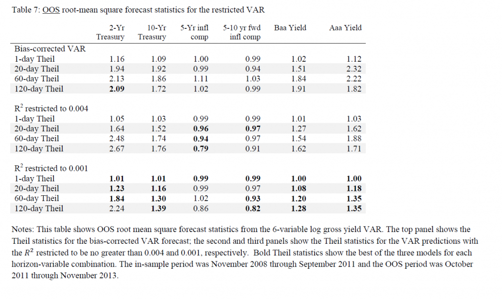
Naive

When the ratio is 1 or greater, this means that the mean square forecast error of the VAR is greater than the benchmark model.

Reflections

There are many fascinating details of these papers I am not highlighting. As an old Republican Congressman once said, “a billion here and a billion there, and pretty soon you are spending real money.”

So the defense of QE in this instance boils down to invalidating an analysis which suggests the impacts of QE are transitory, lasting a few months.

There is no proof, however, that QE has imparted lasting impacts on long term interest rates developed in this relatively recent research.

Forecasting Housing Markets – 2

I am interested in business forecasting “stories.” For example, the glitch in Google’s flu forecasting program.

In real estate forecasting, the obvious thing is whether quantitative forecasting models can (or, better yet, did) forecast the collapse in housing prices and starts in the recent 2008-2010 recession (see graphics from the previous post).

There are several ways of going at this.

Who Saw The Housing Bubble Coming?

One is to look back to see whether anyone saw the bursting of the housing bubble coming and what forecasting models they were consulting.

That’s entertaining. Some people, like Ron Paul, and Nouriel Roubini, were prescient.

Roubini earned the soubriquet Dr. Doom for an early prediction of housing market collapse, as reported by the New York Times:

On Sept. 7, 2006, Nouriel Roubini, an economics professor at New York University, stood before an audience of economists at the International Monetary Fund and announced that a crisis was brewing. In the coming months and years, he warned, the United States was likely to face a once-in-a-lifetime housing bust, an oil shock, sharply declining consumer confidence and, ultimately, a deep recession. He laid out a bleak sequence of events: homeowners defaulting on mortgages, trillions of dollars of mortgage-backed securities unraveling worldwide and the global financial system shuddering to a halt. These developments, he went on, could cripple or destroy hedge funds, investment banks and other major financial institutions like Fannie Mae and Freddie Mac.

NR

Roubini was spot-on, of course, even though, at the time, jokes circulated such as “even a broken clock is right twice a day.” And my guess is his forecasting model, so to speak, is presented in Crisis Economics: A Crash Course in the Future of Finance, his 2010 book with Stephen Mihm. It is less a model than whole database of tendencies, institutional facts, areas in which Roubini correctly identifies moral hazard.

I think Ron Paul, whose projections of collapse came earlier (2003), was operating from some type of libertarian economic model.  So Paul testified before House Financial Services Committee on Fannie Mae and Freddy Mac, that –

Ironically, by transferring the risk of a widespread mortgage default, the government increases the likelihood of a painful crash in the housing market,” Paul predicted. “This is because the special privileges granted to Fannie and Freddie have distorted the housing market by allowing them to attract capital they could not attract under pure market conditions. As a result, capital is diverted from its most productive use into housing. This reduces the efficacy of the entire market and thus reduces the standard of living of all Americans.

On the other hand, there is Ben Bernanke, who in a CNBC interview in 2005 said:

7/1/05 – Interview on CNBC 

INTERVIEWER: Ben, there’s been a lot of talk about a housing bubble, particularly, you know [inaudible] from all sorts of places. Can you give us your view as to whether or not there is a housing bubble out there?

BERNANKE: Well, unquestionably, housing prices are up quite a bit; I think it’s important to note that fundamentals are also very strong. We’ve got a growing economy, jobs, incomes. We’ve got very low mortgage rates. We’ve got demographics supporting housing growth. We’ve got restricted supply in some places. So it’s certainly understandable that prices would go up some. I don’t know whether prices are exactly where they should be, but I think it’s fair to say that much of what’s happened is supported by the strength of the economy.

Bernanke was backed by one of the most far-reaching economic data collection and analysis operations in the United States, since he was in 2005 a member of the Board of Governors of the Federal Reserve System and Chairman of the President’s Council of Economic Advisors.

So that’s kind of how it is. Outsiders, like Roubini and perhaps Paul, make the correct call, but highly respected and well-placed insiders like Bernanke simply cannot interpret the data at their fingertips to suggest that a massive bubble was underway.

I think it is interesting currently that Roubini, in March, promoted the idea that Yellen Is Creating another huge Bubble in the Economy

But What Are the Quantitative Models For Forecasting the Housing Market?

In a long article in the New York Times in 2009, How Did Economists Get It So Wrong?, Paul Krugman lays the problem at the feet of the efficient market hypothesis –

When it comes to the all-too-human problem of recessions and depressions, economists need to abandon the neat but wrong solution of assuming that everyone is rational and markets work perfectly.

Along these lines, it is interesting that the Zillow home value forecast methodology builds on research which, in one set of models, assumes serial correlation and mean reversion to a long-term price trend.

Zillow

Key research in housing market dynamics includes Case and Shiller (1989) and Capozza et al (2004), who show that the housing market is not efficient and house prices exhibit strong serial correlation and mean reversion, where large market swings are usually followed by reversals to the unobserved fundamental price levels.

Based on the estimated model parameters, Capozza et al are able to reveal the housing market characteristics where serial correlation, mean reversion, and oscillatory, convergent, or divergent trends can be derived from the model parameters.

Here is an abstract from critical research underlying this approach done in 2004.

An Anatomy of Price Dynamics in Illiquid Markets: Analysis and Evidence from Local Housing Markets

This research analyzes the dynamic properties of the difference equation that arises when markets exhibit serial correlation and mean reversion. We identify the correlation and reversion parameters for which prices will overshoot equilibrium (“cycles”) and/or diverge permanently from equilibrium. We then estimate the serial correlation and mean reversion coefficients from a large panel data set of 62 metro areas from 1979 to 1995 conditional on a set of economic variables that proxy for information costs, supply costs and expectations. Serial correlation is higher in metro areas with higher real incomes, population growth and real construction costs. Mean reversion is greater in large metro areas and faster growing cities with lower construction costs. The average fitted values for mean reversion and serial correlation lie in the convergent oscillatory region, but specific observations fall in both the damped and oscillatory regions and in both the convergent and divergent regions. Thus, the dynamic properties of housing markets are specific to the given time and location being considered.

The article is not available for free download so far as I can determine. But it is based on earler research, dating back to the later 1990’s in the pdf The Dynamic Structure of Housing Markets.

The more recent Housing Market Dynamics: Evidence of Mean Reversion and Downward Rigidity by Fannie Mae researchers, lists a lot of relevant research on the serial correlation of housing prices, which is usually locality-dependent.

In fact, the Zillow forecasts are based on ensemble methods, combining univariate and multivariate models – a sign of modernity in the era of Big Data.

So far, though, I have not found a truly retrospective study of the housing market collapse, based on quantitative models. Perhaps that is because only the Roubini approach works with such complex global market phenomena.

We are left, thus, with solid theoretical foundations, validated by multiple housing databases over different time periods, that suggests that people invest in housing based on momentum factors – and that this fairly obvious observation can be shown statistically, too.

And Now – David Stockman

David Stockman, according to his new website Contra Corner,

is the ultimate Washington insider turned iconoclast. He began his career in Washington as a young man and quickly rose through the ranks of the Republican Party to become the Director of the Office of Management and Budget under President Ronald Reagan. After leaving the White House, Stockman had a 20-year career on Wall Street.

Currently, Stockman takes the contrarian view that the US Federal Reserve Bank is feeding a giant bubble which is bound to collapse

He states his opinions with humor and wit, as some of article titles on Contra Corner indicate –

Fed’s Taper Kabuki is Farce; Gong Show of Cacophony, Confusion and Calamity Coming

Or

General John McCain Strikes Again!

Forecasting Gold Prices – Goldman Sachs Hits One Out of the Park

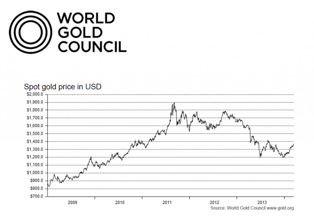
March 25, 2009, Goldman Sachs’ Commodity and Strategy Research group published Global Economics Paper No 183: Forecasting Gold as a Commodity.

This offers a fascinating overview of supply and demand in global gold markets and an immediate prediction –

This “gold as a commodity” framework suggests that gold prices have strong support at and above current price levels should the current low real interest rate environment persist. Specifically, assuming real interest rates stay near current levels and the buying from gold-ETFs slows to last year’s pace, we would expect to see gold prices stay near $930/toz over the next six months, rising to $962/toz on a 12-month horizon.

The World Gold Council maintains an interactive graph of gold prices based on the London PM fix.

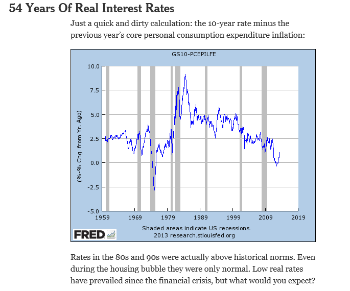
GoldpriceNow, of course, the real interest rate is an inflation-adjusted nominal interest rate. It’s usually estimated as a difference between some representative interest rate and relevant rate of inflation. Thus, the real interest rates in the Goldman Sachs report is really an extrapolation from extant data provided, for example, by the US Federal Reserve FRED database.

Gratis of Paul Krugman’s New York Times blog from last August, we have this time series for real interest rates –

realinterestrates

The graph shows that “real interest rates stay near current levels” (from spring 2009), putting the Goldman Sachs group authoring Report No 183 on record as producing one of the most successful longer term forecasts that you can find.

I’ve been collecting materials on forecasting systems for gold prices, and hope to visit that topic in coming posts here.

Three Pass Regression Filter – New Data Reduction Method

Malcolm Gladwell’s 10,000 hour rule (for cognitive mastery) is sort of an inspiration for me. I picked forecasting as my field for “cognitive mastery,” as dubious as that might be. When I am directly engaged in an assignment, at some point or other, I feel the need for immersion in the data and in estimations of all types. This blog, on the other hand, represents an effort to survey and, to some extent, get control of new “tools” – at least in a first pass. Then, when I have problems at hand, I can try some of these new techniques.

Ok, so these remarks preface what you might call the humility of my approach to new methods currently being innovated. I am not putting myself on a level with the innovators, for example. At the same time, it’s important to retain perspective and not drop a critical stance.

The Working Paper and Article in the Journal of Finance

Probably one of the most widely-cited recent working papers is Kelly and Pruitt’s three pass regression filter (3PRF). The authors, shown above, are with the University of Chicago, Booth School of Business and the Federal Reserve Board of Governors, respectively, and judging from the extensive revisions to the 2011 version, they had a bit of trouble getting this one out of the skunk works.

Recently, however, Kelly and Pruit published an important article in the prestigious Journal of Finance called Market Expectations in the Cross-Section of Present Values. This article applies a version of the three pass regression filter to show that returns and cash flow growth for the aggregate U.S. stock market are highly and robustly predictable.

I learned of a published application of the 3PRF from Francis X. Dieblod’s blog, No Hesitations, where Diebold – one of the most published authorities on forecasting – writes

Recent interesting work, moreover, extends PLS in powerful ways, as with the Kelly-Pruitt three-pass regression filter and its amazing apparent success in predicting aggregate equity returns.

What is the 3PRF?

The working paper from the Booth School of Business cited at a couple of points above describes what might be cast as a generalization of partial least squares (PLS). Certainly, the focus in the 3PRF and PLS is on using latent variables to predict some target.

I’m not sure, though, whether 3PRF is, in fact, more of a heuristic, rather than an algorithm.

What I mean is that the three pass regression filter involves a procedure, described below.

(click to enlarge).
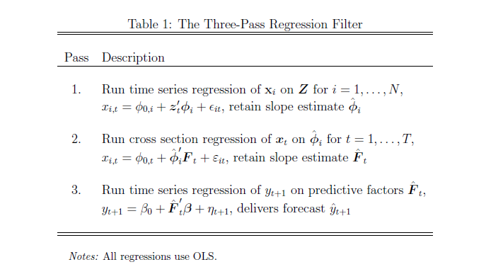
3PRFprocedure

Here’s the basic idea –

Suppose you have a large number of potential regressors xi ε X, i=1,..,N. In fact, it may be impossible to calculate an OLS regression, since N > T the number of observations or time periods.

Furthermore, you have proxies zj ε  Z, I = 1,..,L – where L is significantly less than the number of observations T. These proxies could be the first several principal components of the data matrix, or underlying drivers which theory proposes for the situation. The authors even suggest an automatic procedure for generating proxies in the paper.

And, finally, there is the target variable yt which is a column vector with T observations.

Latent factors in a matrix F drive both the proxies in Z and the predictors in X. Based on macroeconomic research into dynamic factors, there might be only a few of these latent factors – just as typically only a few principal components account for the bulk of variation in a data matrix.

Now here is a key point – as Kelly and Pruitt present the 3PRF, it is a leading indicator approach when applied to forecasting macroeconomic variables such as GDP, inflation, or the like. Thus, the time index for yt ranges from 2,3,…T+1, while the time indices of all X and Z variables and the factors range from 1,2,..T. This means really that all the x and z variables are potentially leading indicators, since they map conditions from an earlier time onto values of a target variable at a subsequent time.

What Table 1 above tells us to do is –

  1. Run an ordinary least square (OLS) regression of the xi      in X onto the zj in X, where T ranges from 1 to T and there are      N variables in X and L << T variables in Z. So, in the example      discussed below, we concoct a spreadsheet example with 3 variables in Z,      or three proxies, and 10 predictor variables xi in X (I could      have used 50, but I wanted to see whether the method worked with lower      dimensionality). The example assumes 40 periods, so t = 1,…,40. There will      be 40 different sets of coefficients of the zj as a result of      estimating these regressions with 40 matched constant terms.
  2. OK, then we take this stack of estimates of      coefficients of the zj and their associated constants and map      them onto the cross sectional slices of X for t = 1,..,T. This means that,      at each period t, the values of the cross-section. xi,t, are      taken as the dependent variable, and the independent variables are the 40      sets of coefficients (plus constant) estimated in the previous step for      period t become the predictors.
  3. Finally, we extract the estimate of the factor loadings      which results, and use these in a regression with target variable as the      dependent variable.

This is tricky, and I have questions about the symbolism in Kelly and Pruitt’s papers, but the procedure they describe does work. There is some Matlab code here alongside the reference to this paper in Professor Kelly’s research.

At the same time, all this can be short-circuited (if you have adequate data without a lot of missing values, apparently) by a single humungous formula –
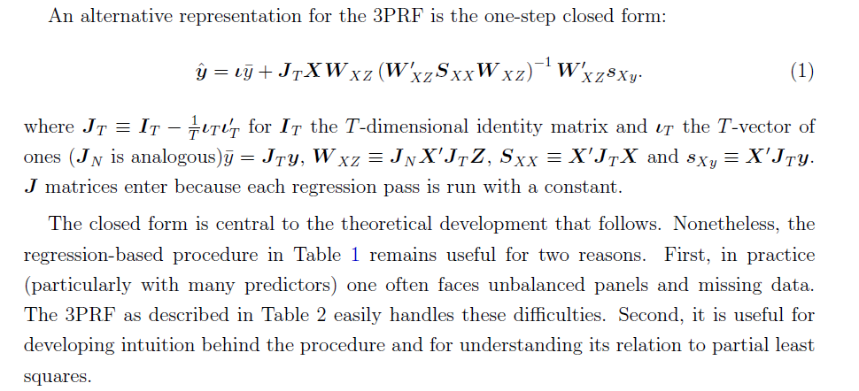
3PRFformula

Here, the source is the 2012 paper.

Spreadsheet Implementation

Spreadsheets help me understand the structure of the underlying data and the order of calculation, even if, for the most part, I work with toy examples.

So recently, I’ve been working through the 3PRF with a small spreadsheet.

Generating the factors:I generated the factors as two columns of random variables (=rand()) in Excel. I gave the factors different magnitudes by multiplying by different constants.

Generating the proxies Z and predictors X. Kelly and Pruitt call for the predictors to be variance standardized, so I generated 40 observations on ten sets of xi by selecting ten different coefficients to multiply into the two factors, and in each case I added a normal error term with mean zero and standard deviation 1. In Excel, this is the formula =norminv(rand(),0,1).

Basically, I did the same drill for the three zj — I created 40 observations for z1, z2, and z3 by multiplying three different sets of coefficients into the two factors and added a normal error term with zero mean and variance equal to 1.

Then, finally, I created yt by multiplying randomly selected coefficients times the factors.

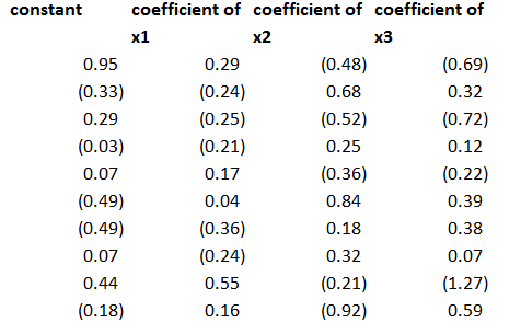
After generating the data, the first pass regression is easy. You just develop a regression with each predictor xi as the dependent variable and the three proxies as the independent variables, case-by-case, across the time series for each. This gives you a bunch of regression coefficients which, in turn, become the explanatory variables in the cross-sectional regressions of the second step.

The regression coefficients I calculated for the three proxies, including a constant term, were as follows – where the 1st row indicates the regression for x1 and so forth.
coeff

This second step is a little tricky, but you just take all the values of the predictor variables for a particular period and designate these as the dependent variables, with the constant and coefficients estimated in the previous step as the independent variables. Note, the number of predictors pairs up exactly with the number of rows in the above coefficient matrix.

This then gives you the factor loadings for the third step, where you can actually predict yt (really yt+1 in the 3PRF setup). The only wrinkle is you don’t use the constant terms estimated in the second step, on the grounds that these reflect “idiosyncratic” effects, according to the 2011 revision of the paper.

Note the authors describe this as a time series approach, but do not indicate how to get around some of the classic pitfalls of regression in a time series context. Obviously, first differencing might be necessary for nonstationary time series like GDP, and other data massaging might be in order.

Bottom line – this worked well in my first implementation.

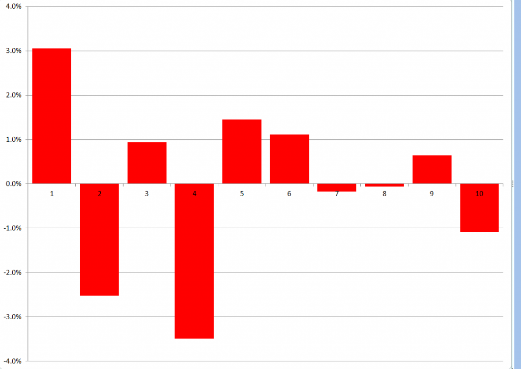
To forecast, I just used the last regression for yt+1 and then added ten more cases, calculating new values for the target variable with the new values of the factors. I used the new values of the predictors to update the second step estimate of factor loadings, and applied the last third pass regression to these values.

Here are the forecast errors for these ten out-of-sample cases.
3PRFforecasterror

Not bad for a first implementation.

 Why Is Three Pass Regression Important?

3PRF is a fairly “clean” solution to an important problem, relating to the issue of “many predictors” in macroeconomics and other business research.

Noting that if the predictors number near or more than the number of observations, the standard ordinary least squares (OLS) forecaster is known to be poorly behaved or nonexistent, the authors write,

How, then, does one effectively use vast predictive information? A solution well known in the economics literature views the data as generated from a model in which latent factors drive the systematic variation of both the forecast target, y, and the matrix of predictors, X. In this setting, the best prediction of y is infeasible since the factors are unobserved. As a result, a factor estimation step is required. The literature’s benchmark method extracts factors that are significant drivers of variation in X and then uses these to forecast y. Our procedure springs from the idea that the factors that are relevant to y may be a strict subset of all the factors driving X. Our method, called the three-pass regression filter (3PRF), selectively identifies only the subset of factors that influence the forecast target while discarding factors that are irrelevant for the target but that may be pervasive among predictors. The 3PRF has the advantage of being expressed in closed form and virtually instantaneous to compute.

So, there are several advantages, such as (1) the solution can be expressed in closed form (in fact as one complicated but easily computable matrix expression), and (2) there is no need to employ maximum likelihood estimation.

Furthermore, 3PRF may outperform other approaches, such as principal components regression or partial least squares.

The paper illustrates the forecasting performance of 3PRF with real-world examples (as well as simulations). The first relates to forecasts of macroeconomic variables using data such as from the Mark Watson database mentioned previously in this blog. The second application relates to predicting asset prices, based on a factor model that ties individual assets’ price-dividend ratios to aggregate stock market fluctuations in order to uncover investors’ discount rates and dividend growth expectations.


Complete Subset Regressions

A couple of years or so ago, I analyzed a software customer satisfaction survey, focusing on larger corporate users. I had firmagraphics – specifying customer features (size, market segment) – and customer evaluation of product features and support, as well as technical training. Altogether, there were 200 questions that translated into metrics or variables, along with measures of customer satisfaction. Altogether, the survey elicited responses from about 5000 companies.

Now this is really sort of an Ur-problem for me. How do you discover relationships in this sort of data space? How do you pick out the most important variables?

Since researching this blog, I’ve learned a lot about this problem. And one of the more fascinating approaches is the recent development named complete subset regressions.

And before describing some Monte Carlo exploring this approach here, I’m pleased Elliot, Gargano, and Timmerman (EGT) validate an intuition I had with this “Ur-problem.” In the survey I mentioned above, I calculated a whole bunch of univariate regressions with customer satisfaction as the dependent variable and each questionnaire variable as the explanatory variable – sort of one step beyond calculating simple correlations. Then, it occurred to me that I might combine all these 200 simple regressions into a predictive relationship. To my surprise, EGT’s research indicates that might have worked, but not be as effective as complete subset regression.

Complete Subset Regression (CSR) Procedure

As I understand it, the idea behind CSR is you run regressions with all possible combinations of some number r less than the total number n of candidate or possible predictors. The final prediction is developed as a simple average of the forecasts from these regressions with r predictors. While some of these regressions may exhibit bias due to specification error and covariance between included and omitted variables, these biases tend to average out, when the right number r < n is selected.

So, maybe you have a database with m observations or cases on some target variable and n predictors.

And you are in the dark as to which of these n predictors or potential explanatory variables really do relate to the target variable.

That is, in a regression y = β01 x1 +…+βn xn some of the beta coefficients may in fact be zero, since there may be zero influence between the associated xi and the target variable y.

Of course, calling all the n variables xi i=1,…n “predictor variables” presupposes more than we know initially. Some of the xi could in fact be “irrelevant variables” with no influence on y.

In a nutshell, the CSR procedure involves taking all possible combinations of some subset r of the n total number of potential predictor variables in the database, and mapping or regressing all these possible combinations onto the dependent variable y. Then, for prediction, an average of the forecasts of all these regressions is often a better predictor than can be generated by other methods – such as the LASSO or bagging.

EGT offer a time series example as an empirical application. based on stock returns, quarterly from 1947-2010 and twelve (12) predictors. The authors determine that the best results are obtained with a small subset of the twelve predictors, and compare these results with ridge regression, bagging, Lasso and Bayesian Model Averaging.

The article in The Journal of Econometrics is well-worth purchasing, if you are not a subscriber. Otherwise, there is a draft in PDF format from 2012.

The combination of n things taken r at a time is n!/[(n-r)!(r!)] and increases faster than exponentially, as n increases. For large n, accordingly, it is necessary to sample from the possible set of combinations – a procedure which still can generate improvements in forecast accuracy over a “kitchen sink” regression (under circumstances further delineated below). Otherwise, you need a quantum computer to process very fat databases.

When CSR Works Best – Professor Elloitt

I had email correspondence with Professor Graham Elliott, one of the co-authors of the above-cited paper in the Journal of Econometrics.

His recommendation is that CSR works best with when there are “weak predictors” sort of buried among a superset of candidate variables,

If a few (say 3) of the variables have large coefficients such as that they result in a relatively large R-square for the prediction regression when they are all included, then CSR is not likely to be the best approach. In this case model selection has a high chance of finding a decent model, the kitchen sink model is not all that much worse (about 3/T times the variance of the residual where T is the sample size) and CSR is likely to be not that great… When there is clear evidence that a predictor should be included then it should be always included…, rather than sometimes as in our method. You will notice that in section 2.3 of the paper that we construct properties where beta is local to zero – what this math says in reality is that we mean the situation where there is very little clear evidence that any predictor is useful but we believe that some or all have some minor predictive ability (the stock market example is a clear case of this). This is the situation where we expect the method to work well. ..But at the end of the day, there is no perfect method for all situations.

I have been toying with “hidden variables” and, then, measurement error in the predictor variables in simulations that further validate Graham Elliot’s perspective that CSR works best with “weak predictors.”

Monte Carlo Simulation

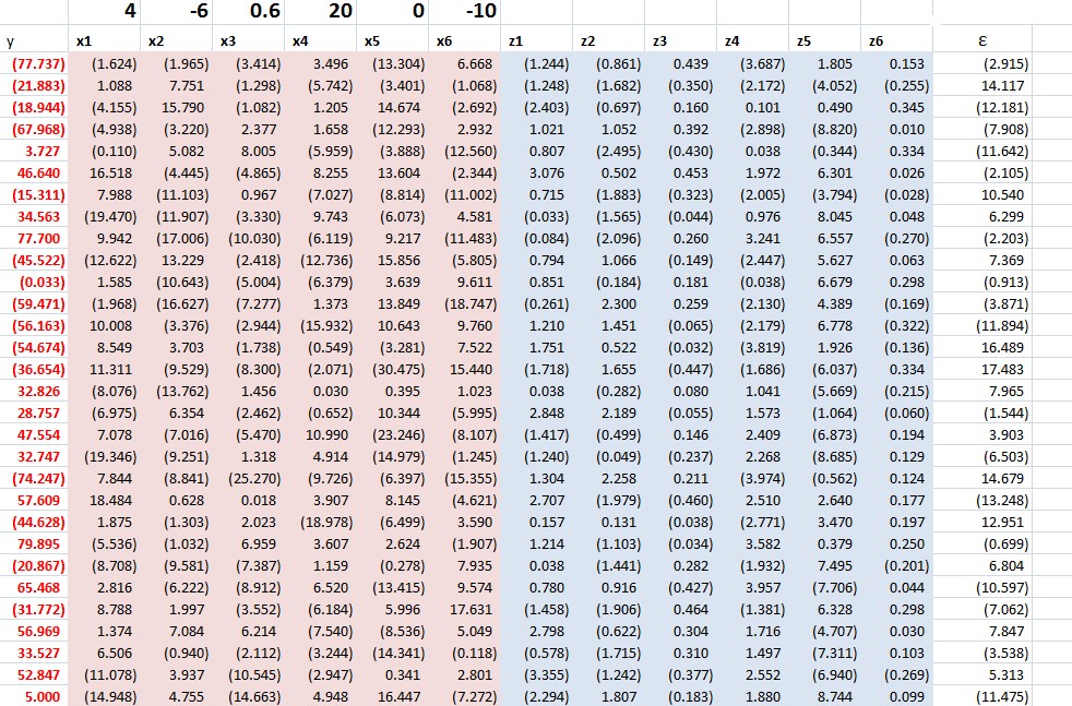
Here’s the spreadsheet for a relevant simulation (click to enlarge).

CSRTable

It is pretty easy to understand this spreadsheet, but it may take a few seconds. It is a case of latent variables, or underlying variables disguised by measurement error.

The z values determine the y value. The z values are multiplied by the bold face numbers in the top row, added together, and then the epsilon error ε value is added to this sum of terms to get each y value. You have to associate the first bold face coefficient with the first z variable, and so forth.

At the same time, an observer only has the x values at his or her disposal to estimate a predictive relationship.

These x variables are generated by adding a Gaussian error to the corresponding value of the z variables.

Note that z5 is an irrelevant variable, since its coefficient loading is zero.

This is a measurement error situation (see the lecture notes on “measurement error in X variables” ).

The relationship with all six regressors – the so-called “kitchen-sink” regression – clearly shows a situation of “weak predictors.”

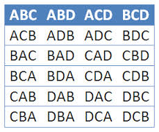
I consider all possible combinations of these 6 variables, taken 3 at a time, or 20 possible distinct combinations of regressors and resulting regressions.

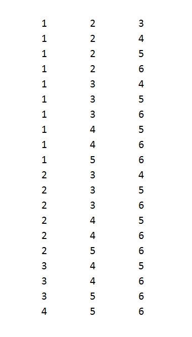
In terms of the mechanics of doing this, it’s helpful to set up the following type of listing of the combinations.

Combos

Each digit in the above numbers indicates a variable to include. So 123 indicates a regression with y and x1, x2, and x3. Note that writing the combinations in this way so they look like numbers in order of increasing size can be done by a simple algorithm for any r and n.

And I can generate thousands of cases by allowing the epsilon ε values and other random errors to vary.

In the specific run above, the CSR average soundly beats the mean square error (MSE) of this full specification in forecasts over ten out-of-sample values. The MSE of the kitchen sink regression, thus, is 2,440 while the MSE of the regression specifying all six regressors is 2653. It’s also true that picking the lowest within-sample MSE among the 20 possible combinations for k = 3 does not produce a lower MSE in the out-of-sample run.

This is characteristics of results in other draws of the random elements. I hesitate to characterize the totality without further studying the requirements for the number of runs, given the variances, and so forth.

I think CSR is exciting research, and hope to learn more about these procedures and report in future posts.

Didier Sornette – Celebrity Bubble Forecaster

Professor Didier Sornette, who holds the Chair in Entreprenuerial Risks at ETH Zurich, is an important thinker, and it is heartening to learn the American Association for the Advancement of Science (AAAS) is electing Professor Sornette a Fellow.

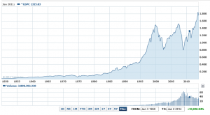
It is impossible to look at, say, the historical performance of the S&P 500 over the past several decades, without concluding that, at some point, the current surge in the market will collapse, as it has done previously when valuations ramped up so rapidly and so far.

S&P500recent

Sornette focuses on asset bubbles and has since 1998, even authoring a book in 2004 on the stock market.

At the same time, I think it is fair to say that he has been largely ignored by mainstream economics (although not finance), perhaps because his training is in physical science. Indeed, many of his publications are in physics journals – which is interesting, but justified because complex systems dynamics cross the boundaries of many subject areas and sciences.

Over the past year or so, I have perused dozens of Sornette papers, many from the extensive list at http://www.er.ethz.ch/publications/finance/bubbles_empirical.

This list is so long and, at times, technical, that videos are welcome.

Along these lines there is Sornette’s Ted talk (see below), and an MP4 file which offers an excellent, high level summary of years of research and findings. This MP4 video was recorded at a talk before the International Center for Mathematical Sciences at the University of Edinburgh.

Intermittent criticality in financial markets: high frequency trading to large-scale bubbles and crashes. You have to download the file to play it.

By way of précis, this presentation offers a high-level summary of the roots of his approach in the economics literature, and highlights the role of a central differential equation for price change in an asset market.

So since I know everyone reading this blog was looking forward to learning about a differential equation, today, let me highlight the importance of the equation,

dp/dt = cpd

This basically says that price change in a market over time depends on the level of prices – a feature of markets where speculative forces begin to hold sway.

This looks to be a fairly simple equation, but the solutions vary, depending on the values of the parameters c and d. For example, when c>0 and the exponent d  is greater than one, prices change faster than exponentially and within some finite period, a singularity is indicated by the solution to the equation. Technically, in the language of differential equations this is called a finite time singularity.

Well, the essence of Sornette’s predictive approach is to estimate the parameters of a price equation that derives, ultimately, from this differential equation in order to predict when an asset market will reach its peak price and then collapse rapidly to lower prices.

The many sources of positive feedback in asset pricing markets are the basis for the faster than exponential growth, resulting from d>1. Lots of empirical evidence backs up the plausibility and credibility of herd and imitative behaviors, and models trace out the interaction of prices with traders motivated by market fundamentals and momentum traders or trend followers.

Interesting new research on this topic shows that random trades could moderate the rush towards collapse in asset markets – possibly offering an alternative to standard regulation.

The important thing, in my opinion, is to discard notions of market efficiency which, even today among some researchers, result in scoffing at the concept of asset bubbles and basic sabotage of research that can help understand the associated dynamics.

Here is a TED talk by Sornette from last summer.

Simulating the SPDR SPY Index

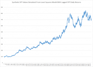
Here is a simulation of the SPDR SPY exchange traded fund index, using an autoregressive model estimated with maximum likehood methods, assuming the underlying distribution is not normal, but is instead a Student t distribution.

SimulatedSPY

The underlying model is of the form

SPYRRt=a0+a1SPYRRt-1…a30SPYRRt-30

Where SPYRR is the daily return (trading day to trading day) of the SPY, based on closing prices.

This is a linear model, and an earlier post lists its exact parameters or, in other words, the coefficients attached to each of the lagged terms, as well as the value of the constant term.

This model is estimated on a training sample of daily returns from 1993 to 2008, and, is applied to out-of-sample data from 2008 to the present. It predicts about 53 percent of the signs of the next-day-returns correctly. The model generates more profits in the 2008 to the present period than a Buy & Hold strategy.

The simulation listed above uses the model equation and parameters, generating a series of 4000 values recursively, adding in randomized error terms from the fit of the equation to the training or estimation data.

This is work-in-progress. Currently, I am thinking about how to properly incorporate volatility. Obviously, any number of realizations are possible. The chart shows one of them, which has an uncanny resemblance to the actual historical series, due to the fact that volatility is created over certain parts of the simulation, in this case by chance.

To review, I set in motion the following process:

  1. Predict a xt = f(xt-1,..,xt-30) based on the 30 coefficients and a constant term from the autoregressive model, applied to 30 preceding values of xt generated by this process (The estimation is initialized with the first 30 actual values of the test data).
  2. Randomly select a residual for this xt based on the empirical distribution of errors from the fit of the predictive relationship to the training set.
  3. Iterate.

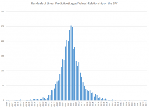
The error distribution looks like this.

MLresidualsSPY

This is obviously not a normal distribution, since “too many” predictive errors are concentrated around the zero error line.

For puzzles and problems, this is a fertile area for research, and you can make money. But obviously, be careful.

In any case, I think this research, in an ultimate analysis, converges to the work being done by Didier Sornette and his co-researchers and co-authors. Sornette et al develop an approach through differential equations, focusing on critical points where a phase shift occurs in trading with a rapid collapse of an asset bubble. 

This approach comes at similar, semi-periodic, logarithmically increasing values through linear autoregressive equations, which, as is well known, have complex dynamics when analyzed as difference equations.

The prejudice in economics and econometrics that “you can’t predict the stock market” is an impediment to integrating these methods. 

While my research on modeling stock prices is a by-product of my general interest in forecasting and quantitative techniques, I may have an advantage because I will try stuff that more seasoned financial analysts may avoid, because they have been told it does not work.

So I maintain it is possible, at least in the era of quantitative easing (QE), to profit from autoregressive models of daily returns on a major index like the SPY. The models are, admittedly, weak predictors, but they interact with the weird error structure of SPY daily returns in interesting ways. And, furthermore, it is possible for anyone to verify my claims simply by calculating the predictions for the test period from 2008 to the present and then looking at what a Buy & Hold Strategy would have done over the same period.

In this post, I reverse the process. I take one of my autoregressive models and generate, by simulation, time series that look like historical SPY daily values.

On Sornette, about which I think we will be hearing more, since currently the US stock market seems to be in correction model, see – Turbulent times ahead: Q&A with economist Didier Sornette. Also check http://www.er.ethz.ch/presentations/index.