Category Archives: predictive analytics

Links – mid-September

After highlighting billionaires by state, I focus on data analytics and marketing, and then IT in these links. Enjoy!

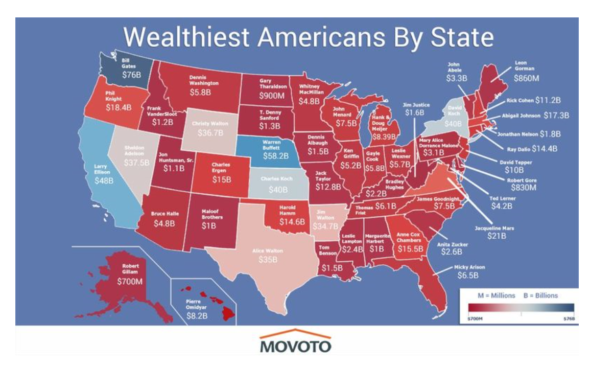
The Wealthiest Individual In Every State [Map]

wealthyindividuals

Data Analytics and Marketing

A Predictive Analytics Primer

Has your company, for example, developed a customer lifetime value (CLTV) measure? That’s using predictive analytics to determine how much a customer will buy from the company over time. Do you have a “next best offer” or product recommendation capability? That’s an analytical prediction of the product or service that your customer is most likely to buy next. Have you made a forecast of next quarter’s sales? Used digital marketing models to determine what ad to place on what publisher’s site? All of these are forms of predictive analytics.

Making sense of Google Analytics audience data

Earlier this year, Google added Demographics and Interest reports to the Audience section of Google Analytics (GA). Now not only can you see how many people are visiting your site, but how old they are, whether they’re male or female, what their interests are, and what they’re in the market for.

Data Visualization, Big Data, and the Quest for Better Decisions – a Synopsis

Simon uses Netflix as a prime example of a company that gets data and its use “to promote experimentation, discovery, and data-informed decision-making among its people.”….

They know a lot about their customers.

For example, the company knows how many people binge-watched the entire season four of Breaking Bad the day before season five came out (50,000 people). The company therefore can extrapolate viewing patterns for its original content produced to appeal to Breaking Bad fans. Moreover, Netflix markets the same show differently to different customers based on whether their viewing history suggests they like the director or one of the stars….

The crux of their analytics is the visualization of “what each streaming customer watches, when, and on what devices, but also at what points shows are paused and resumed (or not) and even the color schemes of the marketing graphics to which individuals respond.”

How to Market Test a New Idea

Formulate a hypothesis to be tested. Determine specific objectives for the test. Make a prediction, even if it is just a wild guess, as to what should happen. Then execute in a way that enables you to accurately measure your prediction…Then involve a dispassionate outsider in the process, ideally one who has learned through experience how to handle decisions with imperfect information…..Avoid considering an idea in isolation. In the absence of choice, you will almost always be able to develop a compelling argument about why to proceed with an innovation project. So instead of asking whether you should invest in a specific project, ask if you are more excited about investing in Project X versus other alternatives in your innovation portfolio…And finally, ensure there is some kind of constraint forcing a decision.

Information Technology (IT)

5 Reasons why Wireless Charging Never Caught on

Charger Bundling, Limited handsets, Time, Portability, and Standardisation – interesting case study topic for IT

Why Jimmy the Robot Means New Opportunities for IT

While Jimmy was created initially for kids, the platform is actually already evolving to be a training platform for everyone. There are two versions: one at $1,600, which really is more focused on kids, and one at $16,000, for folks like us who need a more industrial-grade solution. The Apple I wasn’t just for kids and neither is Jimmy. Consider at least monitoring this effort, if not embracing it, so when robots go vertical you have the skills to ride this wave and not be hit by it.

jimmy-the-robot

Beyond the Reality Distortion Field: A Sober Look at Apple Pay

.. Apple Pay could potentially kick-start the mobile payment business the way the iPod and iTunes launched mobile music 13 years ago. Once again, Apple is leveraging its powerful brand image to bring disparate companies together all in the name of consumer convenience.

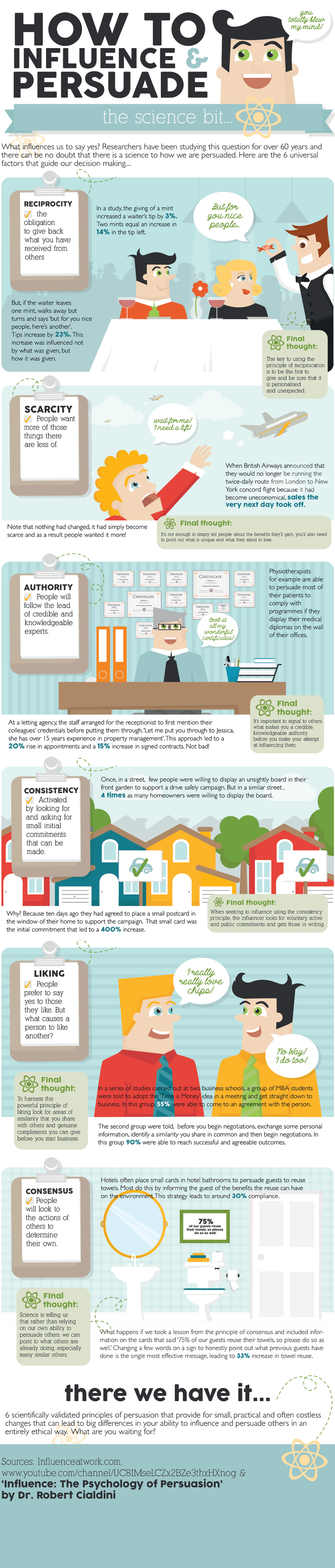
From Dr. 4Ward How To Influence And Persuade (click to enlarge)

influence

Ebola and Data Analysis

Data analysis and predictive analytics can support national and international responses to ebola.

One of the primary ways at present is by verifying and extrapolating the currently exponential growth of ebola in affected areas – especially in Monrovia, the capital of Liberia, as well as Sierra Leone, Guinea, Nigeria, and the Democratic Republic of the Congo.

At this point, given data from the World Health Organization (WHO) and other agencies, predictive modeling can be as simple as in the following two charts, developed from the data compiled (and documented) in the Wikipedia site.

The first charts datapoints from the end of the months of May through August of this year.

Ebolacasesmodeling

The second chart extrapolates an exponential fit to these cases, shown in the lines in the above figure, by month through December 2014.

Ebolaprojections

So by the end of this year, if this epidemic courses unchecked, without the major public health investments necessary in terms of hospital beds, supplies, medical and supporting personnel, including military or police forces to maintain public order in some of the worst-hit areas – there will be nearly 80,000 cases and approximately 30,000 deaths, by this simple extrapolation.

A slightly more sophisticated analysis by Geert Barentsen, utilizing data within calendar months as well, concludes that currently Ebola cases have a doubling time of 29 days.

One possibly positive aspect of these projections is the death rate declines from around 60 to 40 percent, from May through December 2014.

However, if the epidemic continues through 2015 at this rate, the projections suggest there will be more than 300 million cases.

World Health Organization (WHO) estimates released the first week of September indicate nearly 2,400 deaths. Total numbers of cases from the same period in early September is 4,846. So the projections are on track so far.

And, if you wish, you can validate these crude data analytics with reference to modeling using the classic compartment approach and other more advanced setups. See, for example, Disease modelers project a rapidly rising toll from Ebola or the recent New York Times article.

Visual Analytics

There have been advanced modeling efforts at discovering the possibilities of transmission of Ebola through persons traveling by air to other affected areas.

Here is a chart from Assessing the International Spreading Risk Associated with the 2014 West African Ebola Outbreak.

ebolaairroutes

As a data and forecasting analyst, I am not specially equipped to comment on the conditions which make transmission of this disease particularly dangerous. But I think, to some extent, it’s not rocket science.

Crowded conditions in many African cities, low educational attainment, poverty, poor medical infrastructure, rapid population growth – all these factors contribute to the high basic reproductive number of the disease in this outbreak. And, if the numbers of cases increase toward 100,000, the probability that some of the affected individuals will travel elsewhere grows, particularly when efforts to quarantine areas seem heavy-handed and, given little understanding of modern disease models in the affected populations, possibly suspicious.

There is a growing response from agencies and places as widely ranging as the Gates Foundation and Cuba, but what I read is that a military-type operation will be necessary to bring the epidemic under control. I suppose this means command-and-control centers must be established, set procedures must be implemented when cases are identified, adequate field hospitals need to be established, enough medical personnel must be deployed, and so forth. And if there are potential vaccines, these probably will be expensive to administer in early stages.

These thoughts are suggested by the numbers. So far, the numbers speak for themselves.

Links – Labor Day Weekend

Tech

Amazon’s Cloud Is So Pervasive, Even Apple Uses It

Your iCloud storage is apparently on Amazon.

Amazon’s Cloud Is The Fastest Growing Software Business In History

AWS

AWS is Amazon Web Services. The author discounts Google growth, since it is primarily a result of selling advertising. 

How Microsoft and Apple’s Ads Define Their Strategy

Microsoft approaches the market from the top down, while Apple goes after the market from the bottom up.

Mathematical Predictions for the iPhone 6

Can you predict features of the iPhone6 scheduled to be released September 6?

iphoneplot

Predictive Analytics

Comparison of statistical software

Good links for R, Matlab, SAS, Stata, and SPSS.

Types and Uses of Predictive Analytics, What they are and Where You Can Put Them to Work

Gartner says that predictive analytics is a mature technology yet only one company in eight is currently utilizing this ability to predict the future of sales, finance, production, and virtually every other area of the enterprise. What is the promise of predictive analytics and what exactly are they [types and uses of predictive analytics]? Good highlighting of main uses of predictive analytics in companies.

The Four Traps of Predictive Analytics

Magical thinking/ Starting at the Top/ Building Cottages, not Factories/ Seeking Purified Data. Good discussion. This short article in the Sloan Management Review is spot on, in my opinion. The way to develop good predictive analytics is to pick an area, indeed, pick the “low-handing fruit.” Develop workable applications, use them, improve them, broaden the scope. The “throw everything including the kitchen sink” approach of some early Big Data deployments is almost bound to fail. Flashy, trendy, but, in the final analysis, using “exhaust data” to come up with obscure customer metrics probably will not cut in the longer run.

Economic Issues

The Secular Stagnation Controversy

– discusses the e-book Secular Stagnation: Facts, Causes and Cures. The blogger Timothy Taylor points out that “secular” here has no relationship to lacking a religious context, but refers to the idea that market economies, or, if you like, capitalist economies, can experience long periods (decade or more) of desultory economic growth. Check the e-book for Larry Summer’s latest take on the secular stagnation hypothesis.

Here’s how much aid the US wants to send foreign countries in 2015, and why (INFOGRAPHIC

foreignaid

e-commerce and Forecasting

The Census Bureau announced numbers from its latest e-commerce survey August 15.

The basic pattern continues. US retail e-commerce sales increased about 16 percent on a year-over-year basis from the second quarter of 2013. By comparison, total retail sales for the second quarter 2014 increased just short of 5 percent on a year-over-year basis.

 ecommercepercent

As with other government statistics relating to IT (information technology), one can quarrel with the numbers (they may, for example, be low), but there is impressive growth no matter how you cut it.

Some of the top e-retailers from the standpoint of clicks and sales numbers are listed in Panagiotelis et al. Note these are sample data, from comScore with the totals for each company or site representing a small fraction of their actual 2007 online sales.

eretailers

Forecasting Issues

Forecasting issues related to e-commerce run the gamut.

Website optimization and target marketing raise questions such as the profitability of “stickiness” to e-commerce retailers. There are advanced methods to tease out nonlinear, nonnormal multivariate relationships between, say, duration and page views and the decision to purchase – such as copulas previously applied in financial risk assessment and health studies.

Mobile e-commerce is a rapidly growing area with special platform and communications characteristics all its own.

Then, there are the pros and cons of expanding tax collection for online sales.

All in all, Darrell Rigby’s article in the Harvard Business Review – The Future of Shopping – is hard to beat. Traditional retailers generally have to move to a multi-channel model, supplementing brick-and-mortar stores with online services.

I plan several posts on these questions and issues, and am open for your questions.

Top graphic by DIGISECRETS

When the Going Gets Tough, the Tough Get Going

Great phrase, but what does it mean? Well, maybe it has something to do with the fact that a lot of economic and political news seem to be entering kind of “end game.” But, it’s now the “lazy days of summer,” and there is a temptation to sit back and just watch it whiz by.

What are the options?

One is to go more analytical. I’ve recently updated my knowledge base on some esoteric topics –mathematically and analytically interesting – such as kernel ridge regression and dynamic principal components. I’ve previously mentioned these, and there are more instances of analysis to consider. What about them? Are they worth the enormous complexity and computational detail?

Another is to embrace the humming, buzzing confusion and consider “geopolitical risk.” The theme might be the price of oil and impacts, perhaps, of continuing and higher oil prices.

Or the proliferation of open warfare.

Rarely in recent decades have we seen outright armed conflict in Europe, as appears to be on-going in the Ukraine.

And I cannot make much sense of developments in the Mid-East, with some shadowy group called Isis scooping up vast amounts of battlefield armaments abandoned by collapsing Iraqi units.

Or how to understand Israeli bombardment of UN schools in Gaza, and continuing attacks on Israel with drones by Hamas. What is the extent and impact of increasing geopolitical risk?

There also is the issue of plague – most immediately ebola in Africa. A few days ago, I spent the better part of a day in the Boston Airport, and, to pass the time, read the latest Dan Brown book about a diabolical scheme to release an aerosol epidemic of sorts. In any case, ebola is in a way a token of a range of threats that stand just outside the likely. For example, there is the problem of the evolution of immune strains of bacteria, with widespread prescription and use.

There also is the ever-bloating financial bubble that has emerged in the US and elsewhere, as a result of various tactics of central and other banks in reaction to the Great Recession, and behavior of investors.

Finally, there are longer range scientific and technological possibilities. From my standpoint, we are making a hash of things generally. But efforts at political reform, by themselves, usually fall short, unless paralleled by fundamental new possibilities in production or human organization. And the promise of radical innovation for the betterment of things has never seemed brighter.

I will be exploring some of these topics and options in coming posts this week and in coming weeks.

And I think by now I have discovered a personal truth through writing – one that resonates with other experiences of mine professionally and personally. And that is sometimes it is just when the way to going further seems hard to make out that concentration of thought and energies may lead to new insight.

Video Friday – Andrew Ng’s Machine Learning Course

Well, I signed up for Andrew Ng’s Machine Learning Course at Stanford. It began a few weeks ago, and is a next generation to lectures by Ng circulating on YouTube. I’m going to basically audit the course, since I started a little late, but I plan to take several of the exams and work up a few of the projects. This course provides a broad introduction to machine learning, datamining, and statistical pattern recognition. Topics include: (i) Supervised learning (parametric/non-parametric algorithms, support vector machines, kernels, neural networks). (ii) Unsupervised learning (clustering, dimensionality reduction, recommender systems, deep learning). (iii) Best practices in machine learning (bias/variance theory; innovation process in machine learning and AI). The course will also draw from numerous case studies and applications, so that you’ll also learn how to apply learning algorithms to building smart robots (perception, control), text understanding (web search, anti-spam), computer vision, medical informatics, audio, database mining, and other areas. I like the change in format. The YouTube videos circulating on the web are lengthly, and involve Ng doing derivations on white boards. This is a more informal, expository format. Here is a link to a great short introduction to neural networks. Ngrobot Click on the link above this picture, since the picture itself does not trigger a YouTube. Ng’s introduction on this topic is fairly short, so here is the follow-on lecture, which starts the task of representing or modeling neural networks. I really like the way Ng approaches this is grounded in biology. I believe there is still time to sign up. Comment on Neural Networks and Machine Learning I can’t do much better than point to Professor Ng’s definition of machine learning – Machine learning is the science of getting computers to act without being explicitly programmed. In the past decade, machine learning has given us self-driving cars, practical speech recognition, effective web search, and a vastly improved understanding of the human genome. Machine learning is so pervasive today that you probably use it dozens of times a day without knowing it. Many researchers also think it is the best way to make progress towards human-level AI. In this class, you will learn about the most effective machine learning techniques, and gain practice implementing them and getting them to work for yourself. More importantly, you’ll learn about not only the theoretical underpinnings of learning, but also gain the practical know-how needed to quickly and powerfully apply these techniques to new problems. Finally, you’ll learn about some of Silicon Valley’s best practices in innovation as it pertains to machine learning and AI. And now maybe this is the future – the robot rock band.

Wrap on Exponential Smoothing

Here are some notes on essential features of exponential smoothing.

  1. Name. Exponential smoothing (ES) algorithms create exponentially weighted sums of past values to produce the next (and subsequent period) forecasts. So, in simple exponential smoothing, the recursion formula is Lt=αXt+(1-α)Lt-1 where α is the smoothing constant constrained to be within the interval [0,1], Xt is the value of the time series to be forecast in period t, and Lt is the (unobserved) level of the series at period t. Substituting the similar expression for Lt-1 we get Lt=αXt+(1-α) (αXt-1+(1-α)Lt-2)= αXt+α(1-α)Xt-1+(1-α)2Lt-2, and so forth back to L1. This means that more recent values of the time series X are weighted more heavily than values at more distant times in the past. Incidentally, the initial level L1 is not strongly determined, but is established by one ad hoc means or another – often by keying off of the initial values of the X series in some manner or another. In state space formulations, the initial values of the level, trend, and seasonal effects can be included in the list of parameters to be established by maximum likelihood estimation.
  2. Types of Exponential Smoothing Models. ES pivots on a decomposition of time series into level, trend, and seasonal effects. Altogether, there are fifteen ES methods. Each model incorporates a level with the differences coming as to whether the trend and seasonal components or effects exist and whether they are additive or multiplicative; also whether they are damped. In addition to simple exponential smoothing, Holt or two parameter exponential smoothing is another commonly applied model. There are two recursion equations, one for the level Lt and another for the trend Tt, as in the additive formulation, Lt=αXt+(1-α)(Lt-1+Tt-1) and Tt=β(Lt– Lt-1)+(1-β)Tt-1 Here, there are now two smoothing parameters, α and β, each constrained to be in the closed interval [0,1]. Winters or three parameter exponential smoothing, which incorporates seasonal effects, is another popular ES model.
  3. Estimation of the Smoothing Parameters. The original method of estimating the smoothing parameters was to guess their values, following guidelines like “if the smoothing parameter is near 1, past values will be discounted further” and so forth. Thus, if the time series to be forecast was very erratic or variable, a value of the smoothing parameter which was closer to zero might be selected, to achieve a longer period average. The next step is to set up a sum of the squared differences of the within sample predictions and minimize these. Note that the predicted value of Xt+1 in the Holt or two parameter additive case is Lt+Tt, so this involves minimizing the expression Sqerroreq Currently, the most advanced method of estimating the value of the smoothing parameters is to express the model equations in state space form and utilize maximum likelihood estimation. It’s interesting, in this regard, that the error correction version of ES recursion equations are a bridge to this approach, since the error correction formulation is found at the very beginnings of the technique. Advantages of using the state space formulation and maximum likelihood estimation include (a) the ability to estimate confidence intervals for point forecasts, and (b) the capability of extending ES methods to nonlinear models.
  4. Comparison with Box-Jenkins or ARIMA models. ES began as a purely applied method developed for the US Navy, and for a long time was considered an ad hoc procedure. It produced forecasts, but no confidence intervals. In fact, statistical considerations did not enter into the estimation of the smoothing parameters at all, it seemed. That perspective has now changed, and the question is not whether ES has statistical foundations – state space models seem to have solved that. Instead, the tricky issue is to delineate the overlap and differences between ES and ARIMA models. For example, Gardner makes the statement that all linear exponential smoothing methods have equivalent ARIMA models. Hyndman points out that the state space formulation of ES models opens the way for expressing nonlinear time series – a step that goes beyond what is possible in ARIMA modeling.
  5. The Importance of Random Walks. The random walk is a forecasting benchmark. In an early paper, Muth showed that a simple exponential smoothing model provided optimal forecasts for a random walk. The optimal forecast for a simple random walk is the current period value. Things get more complicated when there is an error associated with the latent variable (the level). In that case, the smoothing parameter determines how much of the recent past is allowed to affect the forecast for the next period value.
  6. Random Walks With Drift. A random walk with drift, for which a two parameter ES model can be optimal, is an important form insofar as many business and economic time series appear to be random walks with drift. Thus, first differencing removes the trend, leaving ideally white noise. A huge amount of ink has been spilled in econometric investigations of “unit roots” – essentially exploring whether random walks and random walks with drift are pretty much the whole story when it comes to major economic and business time series.
  7. Advantages of ES. ES is relatively robust, compared with ARIMA models, which are sensitive to mis-specification. Another advantage of ES is that ES forecasts can be up and running with only a few historic observations. This comment applied to estimation of the level and possibly trend, but does not apply in the same degree to the seasonal effects, which usually require more data to establish. There are a number of references which establish the competitive advantage in terms of the accuracy of ES forecasts in a variety of contexts.
  8. Advanced Applications.The most advanced application of ES I have seen is the research paper by Hyndman et al relating to bagging exponential smoothing forecasts.

The bottom line is that anybody interested in and representing competency in business forecasting should spend some time studying the various types of exponential smoothing and the various means to arrive at estimates of their parameters.

For some reason, exponential smoothing reaches deep into actual process in data generation and consistently produces valuable insights into outcomes.

More Blackbox Analysis – ARIMA Modeling in R

Automatic forecasting programs are seductive. They streamline analysis, especially with ARIMA (autoregressive integrated moving average) models. You have to know some basics – such as what the notation ARIMA(2,1,1) or ARIMA(p,d,q) means. But you can more or less sidestep the elaborate algebra – the higher reaches of equations written in backward shift operators – in favor of looking at results. Does the automatic ARIMA model selection predict out-of-sample, for example?

I have been exploring the Hyndman R Forecast package – and other contributors, such as George Athanasopoulos, Slava Razbash, Drew Schmidt, Zhenyu Zhou, Yousaf Khan, Christoph Bergmeir, and Earo Wang, should be mentioned.

A 76 page document lists the routines in Forecast, which you can download as a PDF file.

This post is about the routine auto.arima(.) in the Forecast package. This makes volatility modeling – a place where Box Jenkins or ARIMA modeling is relatively unchallenged – easier. The auto.arima(.) routine also encourages experimentation, and highlights the sharp limitations of volatility modeling in a way that, to my way of thinking, is not at all apparent from the extensive and highly mathematical literature on this topic.

Daily Gold Prices

I grabbed some data from FRED – the Gold Fixing Price set at 10:30 A.M (London time) in London Bullion Market, based in U.S. Dollars.

GOLDAMGBD228NLBM

Now the price series shown in the graph above is a random walk, according to auto.arima(.).

In other words, the routine indicates that the optimal model is ARIMA(0,1,0), which is to say that after differencing the price series once, the program suggests the series reduces to a series of independent random values. The automatic exponential smoothing routine in Forecast is ets(.). Running this confirms that simple exponential smoothing, with a smoothing parameter close to 1, is the optimal model – again, consistent with a random walk.

Here’s a graph of these first differences.

1stdiffgold

But wait, there is a clustering of volatility of these first differences, which can be accentuated if we square these values, producing the following graph.

volatilityGP

Now in a more or less textbook example, auto.arima(.) develops the following ARIMA model for this series

model

Thus, this estimate of the volatility of the first differences of gold price is modeled as a first order autoregressive process with two moving average terms.

Here is the plot of the fitted values.

Rplot1

Nice.

But of course, we are interested in forecasting, and the results here are somewhat more disappointing.

Basically, this type of model makes a horizontal line prediction at a certain level, which is higher when the past values have been higher.

This is what people in quantitative finance call “persistence” but of course sometimes new things happen, and then these types of models do not do well.

From my research on the volatility literature, it seems that short period forecasts are better than longer period forecasts. Ideally, you update your volatility model daily or at even higher frequencies, and it’s likely your one or two period ahead (minutes, hours, a day) will be more accurate.

Incidentally, exponential smoothing in this context appears to be a total fail, again suggesting this series is a simple random walk.

Recapitulation

There is more here than meets the eye.

First, the auto.arima(.) routines in the Hyndman R Forecast package do a competent job of modeling the clustering of higher first differences of the gold price series here. But, at the same time, they highlight a methodological point. The gold price series really has nonlinear aspects that are not adequately commanded by a purely linear model. So, as in many approximations, the assumption of linearity gets us some part of the way, but deeper analysis indicates the existence of nonlinearities. Kind of interesting.

Of course, I have not told you about the notation ARIMA(p,d,q). Well, p stands for the order of the autoregressive terms in the equation, q stands for the moving average terms, and d indicates the times the series is differenced to reduce it to a stationary time series. Take a look at Forecasting: principles and practice – the free forecasting text of Hyndman and Athanasopoulos – in the chapter on ARIMA modeling for more details.

Incidentally, I think it is great that Hyndman and some of his collaborators are providing an open source, indeed free, forecasting package with automatic forecasting capabilities, along with a high quality and, again, free textbook on forecasting to back it up. Eventually, some of these techniques might get dispersed into the general social environment, potentially raising the level of some discussions and thinking about our common future.

And I guess also I have to say that, ultimately, you need to learn the underlying theory and struggle with the algebra some. It can improve one’s ability to model these series.

Microsoft Stock Prices and the Laplace Distribution

The history of science, like the history of all human ideas, is a history of irresponsible dreams, of obstinacy, and of error. But science is one of the very few human activities perhaps the only one in which errors are systematically criticized and fairly often, in time, corrected. This is why we can say that, in science, we often learn from our mistakes, and why we can speak clearly and sensibly about making progress there. — Karl Popper, Conjectures and Refutations

Microsoft daily stock prices and oil futures seem to fall in the same class of distributions as those for the S&P 500 and NASDAQ 100 – what I am calling the Laplace distribution.

This is contrary to the conventional wisdom. The whole thrust of Box-Jenkins time series modeling seems to be to arrive at Gaussian white noise. Most textbooks on econometrics prominently feature normally distributed error processes ~ N(0,σ).

Benoit Mandelbrot, of course, proposed alternatives as far back as the 1960’s, but still we find aggressive application of Gaussian assumptions in applied work – as for example in widespread use of the results of the Black-Scholes theorem or in computing value at risk in portfolios.

Basic Steps

I’m taking a simple approach.

First, I collect daily closing prices for a stock index, stock, or, as you will see, for commodity futures.

Then, I do one of two things: (a) I take the natural logarithms of the daily closing prices, or (b) I simply calculate first differences of the daily closing prices.

I did not favor option (b) initially, because I can show that the first differences, in every case I have looked at, are autocorrelated at various lags. In other words, these differences have an algorithmic structure, although this structure usually has weak explanatory power.

However, it is interesting that the first differences, again in every case I have looked at, are distributed according to one of these sharp-peaked or pointy distributions which are highly symmetric.

Take the daily closing prices of the stock of the Microsoft Corporation (MST), as an example.

Here is a graph of the daily closing prices.

MSFTgraph

And here is a histogram of the raw first differences of those closing prices over this period since 1990.

rawdifMSFT

Now in close reading of The Laplace Distribution and Generalizations I can see there are a range of possibilities in modeling distributions of the above type.

And here is another peaked, relatively symmetric distribution based on the residuals of an autoregressive equation calculated on the first differences of the logarithm of the daily closing prices. That’s a mouthful, but the idea is to extract at least some of the algorithmic component of the first differences.

MSFTregreshisto

That regression is as follows.

MSFTreg

Note the deep depth of the longest lags.

This type of regression, incidentally, makes money in out-of-sample backcasts, although possibly not enough to exceed trading costs unless the size of the trade is large. However, it’s possible that some advanced techniques, such as bagging and boosting, regression trees and random forecasts could enhance the profitability of trading strategies.

Well, a quick look at daily oil futures (CLQ4) from 2007 to the present.

oilfutures

Not quite as symmetric, but still profoundly not a Gaussian distribution.

The Difference It Makes

I’ve got to go back and read Mandelbrot carefully on his analysis of stock and commodity prices. It’s possible that these peaked distributions all fit in a broad class including the Laplace distribution.

But the basic issue here is that the characteristics of these distributions are substantially different than the Gaussian or normal probability distribution. This would affect maximum likelihood estimation of parameters in models, and therefore could affect regression coefficients.

Furthermore, the risk characteristics of assets whose prices have these distributions can be quite different.

And I think there is a moral here about the conventional wisdom and the durability of incorrect ideas.

Top pic is Karl Popper, the philosopher of science