Category Archives: predictive analytics

Partial Least Squares and Principal Components

I’ve run across outstanding summaries of “partial least squares” (PLS) research recently – for example Rosipal and Kramer’s Overview and Recent Advances in Partial Least Squares and the 2010 Handbook of Partial Least Squares.

Partial least squares (PLS) evolved somewhat independently from related statistical techniques, owing to what you might call family connections. The technique was first developed by Swedish statistician Herman Wold and his son, Svante Wold, who applied the method in particular to chemometrics. Rosipal and Kramer suggest that the success of PLS in chemometrics resulted in a lot of applications in other scientific areas including bioinformatics, food research, medicine, [and] pharmacology..

Someday, I want to look into “path modeling” with PLS, but for now, let’s focus on the comparison between PLS regression and principal component (PC) regression. This post develops a comparison with Matlab code and macroeconomics data from Mark Watson’s website at Princeton.

The Basic Idea Behind PC and PLS Regression

Principal component and partial least squares regression share a couple of features.

Both, for example, offer an approach or solution to the problem of “many predictors” and multicollinearity. Also, with both methods, computation is not transparent, in contrast to ordinary least squares (OLS). Both PC and PLS regression are based on iterative or looping algorithms to extract either the principal components or underlying PLS factors and factor loadings.

PC Regression

The first step in PC regression is to calculate the principal components of the data matrix X. This is a set of orthogonal (which is to say completely uncorrelated) vectors which are weighted sums of the predictor variables in X.

This is an iterative process involving transformation of the variance-covariance or correlation matrix to extract the eigenvalues and eigenvectors.

Then, the data matrix X is multiplied by the eigenvectors to obtain the new basis for the data – an orthogonal basis. Typically, the first few (the largest) eigenvalues – which explain the largest proportion of variance in X – and their associated eigenvectors are used to produce one or more principal components which are regressed onto Y. This involves a dimensionality reduction, as well as elimination of potential problems of multicollinearity.

PLS Regression

The basic idea behind PLS regression, on the other hand, is to identify latent factors which explain the variation in both Y and X, then use these factors, which typically are substantially fewer in number than k, to predict Y values.

Clearly, just as in PC regression, the acid test of the model is how it performs on out-of-sample data.

The reason why PLS regression often outperforms PC regression, thus, is that factors which explain the most variation in the data matrix may not, at the same time, explain the most variation in Y. It’s as simple as that.

Matlab example

I grabbed some data from Mark Watson’s website at Princeton — from the links to a recent paper called Generalized Shrinkage Methods for Forecasting Using Many Predictors (with James H. Stock), Journal of Business and Economic Statistics, 30:4 (2012), 481-493.Download Paper (.pdf). Download Supplement (.pdf), Download Data and Replication Files (.zip). The data include the following variables, all expressed as year-over-year (yoy) growth rates: The first variable – real GDP – is taken as the forecasting target. The time periods of all other variables are lagged one period (1 quarter) behind the quarterly values of this target variable.

macrolist

Matlab makes calculation of both principal component and partial least squares regressions easy.

The command to extract principal components is

[coeff, score, latent]=princomp(X)

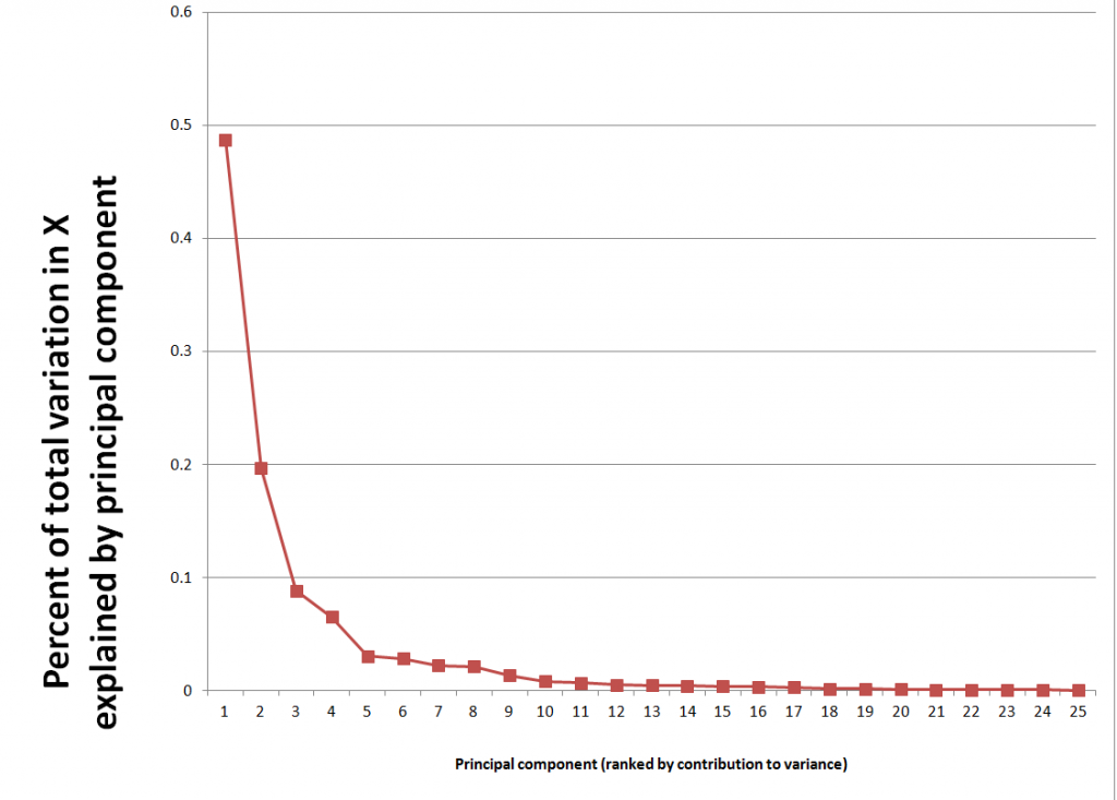
Here X the data matrix, and the entities in the square brackets are vectors or matrices produced by the algorithm. It’s possible to compute a principal components regression with the contents of the matrix score. Generally, the first several principal components are selected for the regression, based on the importance of a component or its associated eigenvalue in latent. The following scree chart illustrates the contribution of the first few principal components to explaining the variance in X.

Screechart

The relevant command for regression in Matlab is

b=regress(Y,score(:,1:6))

where b is the column vector of estimated coefficients and the first six principal components are used in place of the X predictor variables.

The Matlab command for a partial least square regresssion is

[XL,YL,XS,YS,beta] = plsregress(X,Y,ncomp)

where ncomp is the number of latent variables of components to be utilized in the regression. There are issues of interpreting the matrices and vectors in the square brackets, but I used this code –

data=xlsread(‘stock.xls’); X=data(1:47,2:79); y = data(2:48,1);

[XL,yl,XS,YS,beta] = plsregress(X,y,10); yfit = [ones(size(X,1),1) X]*beta;

lookPLS=[y yfit]; ZZ=data(48:50,2:79);newy=data(49:51,1);

new=[ones(3,1) ZZ]*beta; out=[newy new];

The bottom line is to test the estimates of the response coefficients on out-of-sample data.

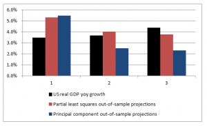
The following chart shows that PLS outperforms PC, although the predictions of both are not spectacularly accurate.

plspccomp

Commentary

There are nuances to what I have done which help explain the dominance of PLS in this situation, as well as the weakly predictive capabilities of both approaches.

First, the target variable is quarterly year-over-year growth of real US GDP. The predictor set X contains 78 other macroeconomic variables, all expressed in terms of yoy (year-over-year) percent changes.

Again, note that the time period of all the variables or observations in X are lagged one quarter from the values in Y, or the values or yoy quarterly percent growth of real US GDP.

This means that we are looking for a real, live leading indicator. Furthermore, there are plausibly common factors in the Y series shared with at least some of the X variables. For example, the percent changes of a block of variables contained in real GDP are included in X, and by inspection move very similarly with the target variable.

Other Example Applications

There are at least a couple of interesting applied papers in the Handbook of Partial Least Squares – a downloadable book in the Springer Handbooks of Computational Statistics. See –

Chapter 20 A PLS Model to Study Brand Preference: An Application to the Mobile Phone Market

Chapter 22 Modeling the Impact of Corporate Reputation on Customer Satisfaction and Loyalty Using Partial Least Squares

Another macroeconomics application from the New York Fed –

“Revisiting Useful Approaches to Data-Rich Macroeconomic Forecasting”

http://www.newyorkfed.org/research/staff_reports/sr327.pdf

Finally, the software company XLStat has a nice, short video on partial least squares regression applied to a marketing example.

Variable Selection Procedures – The LASSO

The LASSO (Least Absolute Shrinkage and Selection Operator) is a method of automatic variable selection which can be used to select predictors X* of a target variable Y from a larger set of potential or candidate predictors X.

Developed in 1996 by Tibshirani, the LASSO formulates curve fitting as a quadratic programming problem, where the objective function penalizes the absolute size of the regression coefficients, based on the value of a tuning parameter λ. In doing so, the LASSO can drive the coefficients of irrelevant variables to zero, thus performing automatic variable selection.

This post features a toy example illustrating tactics in variable selection with the lasso. The post also dicusses the issue of consistency – how we know from a large sample perspective that we are honing in on the true set of predictors when we apply the LASSO.

My take is a two-step approach is often best. The first step is to use the LASSO to identify a subset of potential predictors which are likely to include the best predictors. Then, implement stepwise regression or other standard variable selection procedures to select the final specification, since there is a presumption that the LASSO “over-selects” (Suggested at the end of On Model Selection Consistency of Lasso).

Toy Example

The LASSO penalizes the absolute size of the regression coefficients, based on the value of a tuning parameter λ. When there are many possible predictors, many of which actually exert zero to little influence on a target variable, the lasso can be especially useful in variable selection.

For example, generate a batch of random variables in a 100 by 15 array – representing 100 observations on 15 potential explanatory variables. Mean-center each column. Then, determine coefficient values for these 15 explanatory variables, allowing several to have zero contribution to the dependent variable. Calculate the value of the dependent variable y for each of these 100 cases, adding in a normally distributed error term.

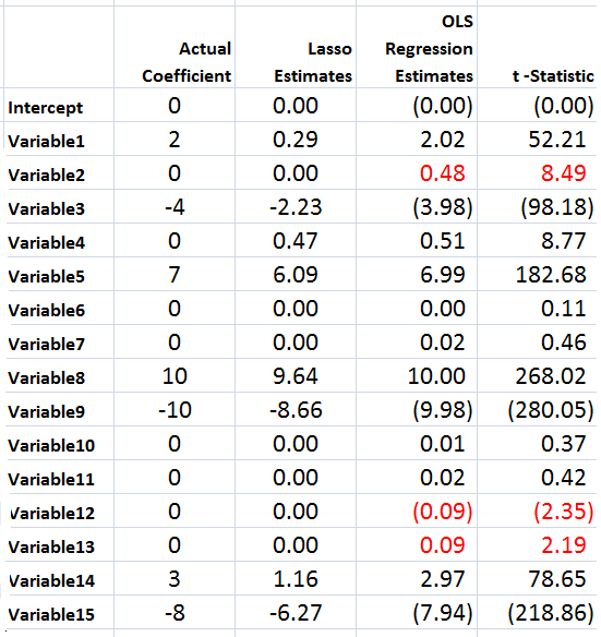
The following Table illustrates something of the power of the lasso.

LassoSS

Using the Matlab lasso procedure and a lambda value of 0.3, seven of the eight zero coefficients are correctly identified. The OLS regression estimate, on the other hand, indicates that three of the zero coefficients are nonzero at a level of 95 percent statistical significance or more (magnitude of the t-statistic > 2).

Of course, the lasso also shrinks the value of the nonzero coefficients. Like ridge regression, then, the lasso introduces bias to parameter estimates, and, indeed, for large enough values of lambda drives all coefficient to zero.

Note OLS can become impossible, when the number of predictors in X* is greater than the number of observations in Y and X. The LASSO, however, has no problem dealing with many predictors.

Real World Examples

For a recent application of the lasso, see the Dallas Federal Reserve occasional paper Hedge Fund Dynamic Market Stability. Note that the lasso is used to identify the key drivers, and other estimation techniques are employed to hone in on the parameter estimates.

For an application of the LASSO to logistic regression in genetics and molecular biology, see Lasso Logistic Regression, GSoft and the Cyclic Coordinate Descent Algorithm, Application to Gene Expression Data. As the title suggests, this illustrates the use of the lasso in logistic regression, frequently utilized in biomedical applications.

Formal Statement of the Problem Solved by the LASSO

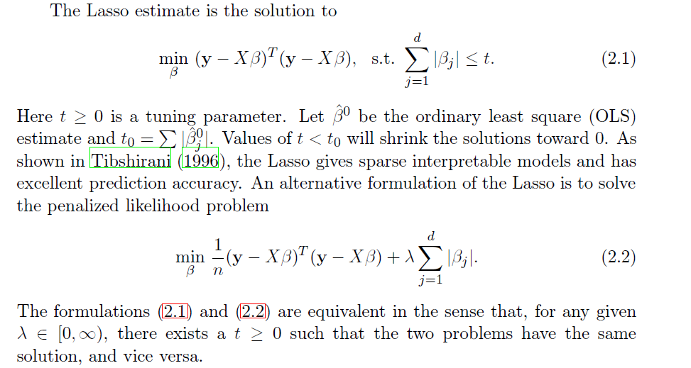
The objective function in the lasso involves minimizing the residual sum of squares, the same entity figuring in ordinary least squares (OLS) regression, subject to a bound on the sum of the absolute value of the coefficients. The following clarifies this in notation, spelling out the objective function.

LassoDerivation

LassoDerivation2

The computation of the lasso solutions is a quadratic programming problem, tackled by standard numerical analysis algorithms. For an analytical discussion of the lasso and other regression shrinkage methods, see the outstanding free textbook The Elements of Statistical Learning by Hastie, Tibshirani, and Friedman.

The Issue of Consistency

The consistency of an estimator or procedure concerns its large sample characteristics. We know the LASSO produces biased parameter estimates, so the relevant consistency is whether the LASSO correctly predicts which variables from a larger set are in fact the predictors.

In other words, when can the LASSO select the “true model?”

Now in the past, this literature is extraordinarily opaque, involving something called the Irrepresentable Condition, which can be glossed as –

almost necessary and sufficient for Lasso to select the true model both in the classical fixed p setting and in the large p setting as the sample size n gets large…This Irrepresentable Condition, which depends mainly on the covariance of the predictor variables, states that Lasso selects the true model consistently if and (almost) only if the predictors that are not in the true model are “irrepresentable” (in a sense to be clarified) by predictors that are in the true model.

Fortunately a ray of light has burst through with Assumptionless Consistency of the Lasso by Chatterjee. Apparently, the LASSO selects the true model almost always – with minimal side assumptions – providing we are satisfied with the prediction error criterion – the mean square prediction error – employed in Tibshirani’s original paper.

Finally, cross-validation is typically used to select the tuning parameter λ, and is another example of this procedure highlighted by Varian’s recent paper.

Using Math to Cure Cancer

There are a couple of takes on this.

One is like “big data and data analytics supplanting doctors.”

So Dr. Cary Oberije certainly knows how to gain popularity with conventional-minded doctors.

In Mathematical Models Out-Perform Doctors in Predicting Cancer Patients’ Responses to Treatment she reports on research showing predictive models are better than doctors at predicting the outcomes and responses of lung cancer patients to treatment… “The number of treatment options available for lung cancer patients are increasing, as well as the amount of information available to the individual patient. It is evident that this will complicate the task of the doctor in the future,” said the presenter, Dr Cary Oberije, a postdoctoral researcher at the MAASTRO Clinic, Maastricht University Medical Center, Maastricht, The Netherlands. “If models based on patient, tumor and treatment characteristics already out-perform the doctors, then it is unethical to make treatment decisions based solely on the doctors’ opinions. We believe models should be implemented in clinical practice to guide decisions.”

 CaryOberije                      

Dr Oberije says,

Correct prediction of outcomes is important for several reasons… First, it offers the possibility to discuss treatment options with patients. If survival chances are very low, some patients might opt for a less aggressive treatment with fewer side-effects and better quality of life. Second, it could be used to assess which patients are eligible for a specific clinical trial. Third, correct predictions make it possible to improve and optimise the treatment. Currently, treatment guidelines are applied to the whole lung cancer population, but we know that some patients are cured while others are not and some patients suffer from severe side-effects while others don’t. We know that there are many factors that play a role in the prognosis of patients and prediction models can combine them all.”

At present, prediction models are not used as widely as they could be by doctors…. some models lack clinical credibility; others have not yet been tested; the models need to be available and easy to use by doctors; and many doctors still think that seeing a patient gives them information that cannot be captured in a model.

Dr. Oberije asserts, Our study shows that it is very unlikely that a doctor can outperform a model.

Along the same lines, mathematical models also have been deployed to predict erectile dysfunction after prostate cancer.

I think Dr. Oberije is probably right that physicians could do well to avail themselves of broader medical databases – on prostate conditions, for example – rather than sort of shooting from the hip with each patient.

The other approach is “teamwork between physicians, data and other analysts should be the goal.”

So it’s with interest I note the Moffit Cancer Center in Tampa Florida espouses a teamwork concept in cancer treatment with new targeted molecular therapies.

page1_clip_image006

The IMO program’s approach is to develop mathematical models and computer simulations to link data that is obtained in a laboratory and the clinic. The models can provide insight into which drugs will or will not work in a clinical setting, and how to design more effective drug administration schedules, especially for drug combinations.  The investigators collaborate with experts in the fields of biology, mathematics, computer science, imaging, and clinical science.

“Limited penetration may be one of the main causes that drugs that showed good therapeutic effect in laboratory experiments fail in clinical trials,” explained Rejniak. “Mathematical modeling can help us understand which tumor, or drug-related factors, hinder the drug penetration process, and how to overcome these obstacles.” 

A similar story cropped up in in the Boston Globe – Harvard researchers use math to find smarter ways to defeat cancer

Now, a new study authored by an unusual combination of Harvard mathematicians and oncologists from leading cancer centers uses modeling to predict how tumors mutate to foil the onslaught of targeted drugs. The study suggests that administering targeted medications one at a time may actually insure that the disease will not be cured. Instead, the study suggests that drugs should be given in combination.

header picture: http://www.en.utexas.edu/Classes/Bremen/e316k/316kprivate/scans/hysteria.html

Tornado Frequency Distribution

Data analysis, data science, and advanced statistics have an important role to play in climate science.

James Elsner’s blog Hurricane & Tornado Climate offers salient examples, in this regard.

Yesterday’s post was motivated by an Elsner suggestion that the time trend in maximum wind speeds of larger or more powerful hurricanes is strongly positive since weather satellite observations provide better measurement (post-1977).

Here’s a powerful, short video illustrating the importance of proper data segmentation and statistical characterization for tornado data – especially for years of tremendous devastation, such as 2011.

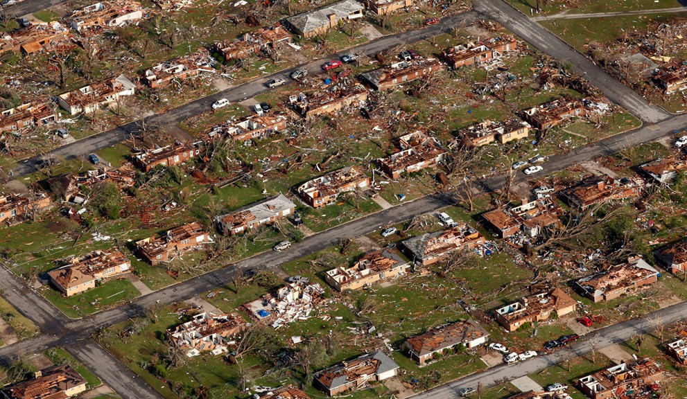
Events that year have a more than academic interest for me, incidentally, since my city of birth – Joplin, Missouri – suffered the effects of a immense supercell which touched down and destroyed everything in its path, including my childhood home. The path of this monster was, at points, nearly a mile wide, and it gouged out a track several miles through this medium size city.

Here is Elsner’s video integrating data analysis with matters of high human import.

There is a sort of extension, in my mind, of the rational expectations issue to impacts of climate change and extreme weather. The question is not exactly one people living in areas subject to these events might welcome. But it is highly relevant to data analysis and statistics.

The question simply is whether US property and other insurance companies are up-to-speed on the type of data segmentation and analysis that is needed to adequately capture the probable future impacts of some of these extreme weather events.

This may be where the rubber hits the road with respect to Bayesian techniques – popular with at least some prominent climate researchers, because they allow inclusion of earlier, less-well documented historical observations.

Quantile Regression

There’s a straight-forward way to understand the value and potential significance of quantile regression – consider the hurricane data referenced in James Elsner’s blog Hurricane & Tornado Climate.

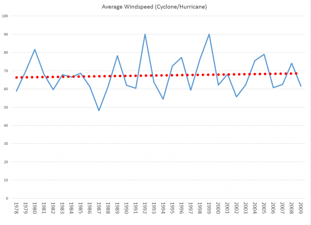
Here is a plot of average windspeed of hurricanes in the Atlantic and Gulf Coast since satellite observations began after 1977.

HurricaneAvgWS

Based on averages, the linear trend line increases about 2 miles per hour over this approximately 30 year period.

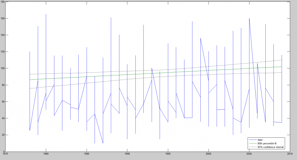
An 80th percentile quantile regression trend line, on the other hand, with this data indicates that the trend in the more violent hurricanes shows an about 15 mph increase over this same period.

HurricaneQuartileReg

In other words, if we look at the hurricanes which are in the 80th percentile or more, there is a much stronger trend in maximum wind speeds, than in the average for all US-related hurricanes in this period.

A quantile q, 0<q<1, splits the data into proportions q below and 1-q above. The most familiar quantile, thus, may be the 50th percentile which is the quantile which splits the data at the median – 50 percent below and 50 percent above.

Quantile regression (QR) was developed, in its modern incarnation by Koenker and Basset in 1978. QR is less influenced by non-normal errors and outliers, and provides a richer characterization of the data.

Thus, QR encourages considering the impact of a covariate on the entire distribution of y, not just is conditional mean.

Roger Koenker and Kevin F. Hallock’s Quantile Regression in the Journal of Economic Perspectives 2001 is a standard reference.

We say that a student scores at the tth quantile of a standardized exam if he performs better than the proportion t of the reference group of students and worse than the proportion (1–t). Thus, half of students perform better than the median student and half perform worse. Similarly, the quartiles divide the population into four segments with equal proportions of the reference population in each segment. The quintiles divide the population into five parts; the deciles into ten parts. The quantiles, or percentiles, or occasionally fractiles, refer to the general case.

Just as we can define the sample mean as the solution to the problem of minimizing a sum of squared residuals, we can define the median as the solution to the problem of minimizing a sum of absolute residuals.

Ordinary least squares (OLS) regression minimizes the sum of squared errors of observations minus estimates. This minimization leads to explicit equations for regression parameters, given standard assumptions.

Quantile regression, on the other hand, minimizes weighted sums of absolute deviations of observations on a quantile minus estimates. This minimization problem is solved by the simplex method of linear programming, rather than differential calculus. The solution is robust to departures from normality of the error process and outliers.

Koenker’s webpage is a valuable resource with directions for available software to estimate QR. I utilized Mathworks Matlab for my estimate of a QR with the hurricane data, along with a supplemental program for quantreg(.) I downloaded from their site.

Here are a couple of short, helpful videos from Econometrics Academy.

Featured image from http://www.huffingtonpost.com/2012/10/29/hurricane-sandy-apps-storm-tracker-weather-channel-red-cross_n_2039433.html

Possibilities for Abrupt Climate Change

The National Research Council (NRC) published ABRUPT IMPACTS OF CLIMATE CHANGE recently, downloadable from the National Academies Press website.

It’s the third NRC report to focus on abrupt climate change, the first being published in 2002. NRC members are drawn from the councils of the National Academy of Sciences, the National Academy of Engineering, and the Institute of Medicine.

The climate change issue is a profound problem in causal discovery and forecasting, to say the very least.

Before I highlight graphic and pictoral resources of the recent NRC report, let me note that Menzie Chin at Econbrowser posted recently on Economic Implications of Anthropogenic Climate Change and Extreme Weather. Chin focuses on the scientific consensus, presenting graphics illustrating the more or less relentless upward march of global average temperatures and estimates (by James Stock no less) of the man-made (anthropogenic) component.

The Econbrowser Comments section is usually interesting and revealing, and this time is no exception. Comments range from “climate change is a left-wing conspiracy” and arguments that “warmer would be better” to the more defensible thought that coming to grips with global climate change would probably mean restructuring our economic setup, its incentives, and so forth.

But I do think the main aspects of the climate change problem – is it real, what are its impacts, what can be done – are amenable to causal analysis at fairly deep levels.

To dispel ideological nonsense, current trends in energy use – growing globally at about 2 percent per annum over a long period – lead to the Earth becoming a small star within two thousand years, or less – generating the amount of energy radiated by the Sun. Of course, changes in energy use trends can be expected before then, when for example the average ambient temperature reaches the boiling point of water, and so forth. These types of calculations also can be made realistically about the proliferation of the automobile culture globally with respect to air pollution and, again, contributions to average temperature. Or one might simply consider the increase in the use of materials and energy for a global population of ten billion, up from today’s number of about 7 billion.

Highlights of the Recent NRC Report

It’s worth quoting the opening paragraph of the report summary –

Levels of carbon dioxide and other greenhouse gases in Earth’s atmosphere are exceeding levels recorded in the past millions of years, and thus climate is being forced beyond the range of the recent geological era. Lacking concerted action by the world’s nations, it is clear that the future climate will be warmer, sea levels will rise, global rainfall patterns will change, and ecosystems will be altered.

So because of growing CO2 (and other greenhouse gases), climate change is underway.

The question considered in ABRUPT IMPACTS OF CLIMATE CHANGE (AICH), however, is whether various thresholds will be crossed, whereby rapid, relatively discontinuous climate change occurs. Such abrupt changes – with radical shifts occurring over decades, rather than centuries – before. AICH thus cites,

..the end of the Younger Dryas, a period of cold climatic conditions and drought in the north that occurred about 12,000 years ago. Following a millennium-long cold period, the Younger Dryas abruptly terminated in a few decades or less and is associated with the extinction of 72 percent of the large-bodied mammals in North America.

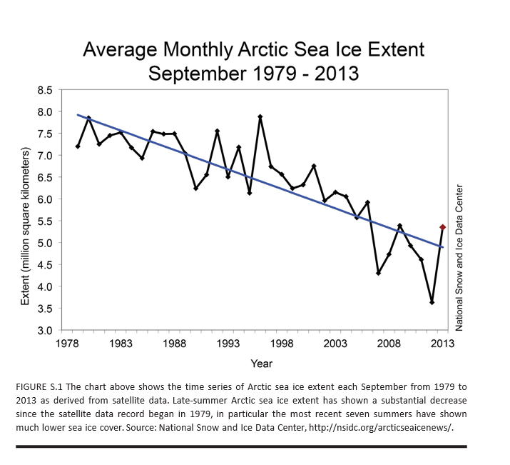
The main abrupt climate change noted in AICH is rapid decline of the Artic sea ice. AICH puts up a chart which is one of the clearest examples of a trend you can pull from environmental science, I would think.

ArticSeaIce

AICH also puts species extinction front and center as a near-term and certain discontinuous effect of current trends.

Apart from melting of the Artic sea ice and species extinction, AICH lists destabilization of the Antarctic ice sheet as a nearer term possibility with dramatic consequences. Because a lot of this ice in the Antarctic is underwater, apparently, it is more at risk than, say, the Greenland ice sheet. Melting of either one (or both) of these ice sheets would raise sea levels tens of meters – an estimated 60 meters with melting of both.

Two other possibilities mentioned in previous NRC reports on abrupt climate change are discussed and evaluated as low probability developments until after 2100. These are stopping of the ocean currents that circulate water in the Atlantic, warming northern Europe, and release of methane from permafrost or deep ocean deposits.

The AMOC is the ocean circulation pattern that involves the northward flow of warm near-surface waters into the northern North Atlantic and Nordic Seas, and the south- ward flow at depth of the cold dense waters formed in those high latitude regions. This circulation pattern plays a critical role in the global transport of oceanic heat, salt, and carbon. Paleoclimate evidence of temperature and other changes recorded in North Atlantic Ocean sediments, Greenland ice cores and other archives suggest that the AMOC abruptly shut down and restarted in the past—possibly triggered by large pulses of glacial meltwater or gradual meltwater supplies crossing a threshold—raising questions about the potential for abrupt change in the future.

Despite these concerns, recent climate and Earth system model simulations indicate that the AMOC is currently stable in the face of likely perturbations, and that an abrupt change will not occur in this century. This is a robust result across many different models, and one that eases some of the concerns about future climate change.

With respect to the methane deposits in Siberia and elsewhere,

Large amounts of carbon are stored at high latitudes in potentially labile reservoirs such as permafrost soils and methane-containing ices called methane hydrate or clathrate, especially offshore in ocean marginal sediments. Owing to their sheer size, these carbon stocks have the potential to massively affect Earth’s climate should they somehow be released to the atmosphere. An abrupt release of methane is particularly worrisome because methane is many times more potent than carbon dioxide as a greenhouse gas over short time scales. Furthermore, methane is oxidized to carbon dioxide in the atmosphere, representing another carbon dioxide pathway from the biosphere to the atmosphere.

According to current scientific understanding, Arctic carbon stores are poised to play a significant amplifying role in the century-scale buildup of carbon dioxide and methane in the atmosphere, but are unlikely to do so abruptly, i.e., on a timescale of one or a few decades. Although comforting, this conclusion is based on immature science and sparse monitoring capabilities. Basic research is required to assess the long-term stability of currently frozen Arctic and sub-Arctic soil stocks, and of the possibility of increasing the release of methane gas bubbles from currently frozen marine and terrestrial sediments, as temperatures rise.

So some bad news and, I suppose, good news – more time to address what would certainly be completely catastrophic to the global economy and world population.

AICH has some neat graphics and pictoral exhibits.

For example, Miami Florida will be largely underwater within a few decades, according to many standard forecasts of increases in sea level (click to enlarge).

Florida

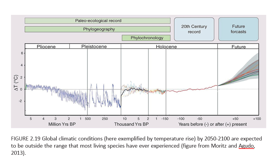
But perhaps most chilling of all (actually not a good metaphor here but you know what I mean) is a graphic I have not seen before, but which dovetails with my initial comments and observations of physicists.

This chart toward the end of the AICH report projects increase in global temperature beyond any past historic level (or prehistoric, for that matter) by the end of the century.

TempRise

So, for sure, there will be species extinction in the near term, hopefully not including the human species just yet.

Economic Impacts

In closing, I do think the primary obstacle to a sober evaluation of climate change involves social and economic implications. The climate change deniers may be right – acknowledging and adequately planning for responses to climate change would involve significant changes in social control and probably economic organization.

Of course, the AICH adopts a more moderate perspective – let’s be sure and set up monitoring of all this, so we can be prepared.

Hopefully, that will happen to some degree.

But adopting a more pro-active stance seems unlikely, at least in the near term. There is a wholesale rush to bringing one to several trillion persons who are basically living in huts with dirt floors into “the modern world.” Their children are traveling to cities, where they will earn much higher incomes, probably, and send money back home. The urge to have a family is almost universal, almost a concomitant of healthy love of a man and a woman. Tradeoffs between economic growth and environmental quality are a tough sell, when there are millions of new consumers and workers to be incorporated into the global supply chain. The developed nations – where energy and pollution output ratios are much better – are not persuasive when they suggest a developing giant like India or China should tow the line, limit energy consumption, throttle back economic growth in order to have a cooler future for the planet. You already got yours Jack, and now you want to cut back? What about mine? As standards of living degrade in the developed world with slower growth there, and as the wealthy grab more power in the situation, garnering even more relative wealth, the political dialogue gets stuck, when it comes to making changes for the good of all.

I could continue, and probably will sometime, but it seems to me that from a longer term forecasting perspective darker scenarios could well be considered. I’m sure we will see quite a few of these. One of the primary ones would be a kind of devolution of the global economy – the sort of thing one might expect if air travel were less possible because of, say, a major uptick in volcanism, or huge droughts took hold in parts of Asia.

Again and again, I come back to the personal thought of local self-reliance. There has been a growth with global supply chains and various centralizations, mergers, and so forth toward de-skilling populations, pushing them into meaningless service sector jobs (fast food), and losing old knowledge about, say, canning fruits and vegetables, or simply growing your own food. This sort of thing has always been a sort of quirky alternative to life in the fast lane. But inasmuch as life in the fast lane involves too much energy use for too many people to pursue, I think decentralized alternatives for lifestyle deserve a serious second look.

Polar bear on ice flow at top from http://metro.co.uk/2010/03/03/polar-bears-cling-to-iceberg-as-climate-change-ruins-their-day-141656/

Causal Discovery

So there’s a new kid on the block, really a former resident who moved back to the neighborhood with spiffy new toys – causal discovery.

Competitions and challenges give a flavor of this rapidly developing field – for example, the Causality Challenge #3: Cause-effect pairs, sponsored by a list of pre-eminent IT organizations and scientific societies (including Kaggle).

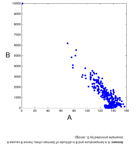
By way of illustration, B → A but A does not cause B – Why?

Kagglealttemp

These data, as the flipped answer indicates, are temperature and altitude of German cities. So altitude causes temperature, but temperature obviously does not cause altitude.

The non-linearity in the scatter diagram is a clue. Thus, values of variable A above about 130 map onto more than one value of B, which is problematic from conventional definition of causality. One cause should not have two completely different effects, unless there are confounding variables.

It’s a little fuzzy, but the associated challenge is very interesting, and data pairs still are available.

We provide hundreds of pairs of real variables with known causal relationships from domains as diverse as chemistry, climatology, ecology, economy, engineering, epidemiology, genomics, medicine, physics. and sociology. Those are intermixed with controls (pairs of independent variables and pairs of variables that are dependent but not causally related) and semi-artificial cause-effect pairs (real variables mixed in various ways to produce a given outcome).  This challenge is limited to pairs of variables deprived of their context.

Asymmetries As Clues to Causal Direction of Influence

The causal direction in the graph above is suggested by the non-invertibility of the functional relationship between B and A.

Another clue from reversing the direction of causal influence relates to the error distributions of the functional relationship between pairs of variables. This occurs when these error distributions are non-Gaussian, as Patrik Hoyer and others illustrate in Nonlinear causal discovery with additive noise models.

The authors present simulation and empirical examples.

Their first real-world example comes from data on eruptions of the Old Faithful geyser in Yellowstone National Park in the US.

OldFaithful Hoyer et al write,

The first dataset, the “Old Faithful” dataset [17] contains data about the duration of an eruption and the time interval between subsequent eruptions of the Old Faithful geyser in Yellowstone National Park, USA. Our method obtains a p-value of 0.5 for the (forward) model “current duration causes next interval length” and a p-value of 4.4 x 10⁻⁹ for the (backward) model “next interval length causes current duration”. Thus, we accept the model where the time interval between the current and the next eruption is a function of the duration of the current eruption, but reject the reverse model. This is in line with the chronological ordering of these events. Figure 3 illustrates the data, the forward and backward fit and the residuals for both fits. Note that for the forward model, the residuals seem to be independent of the duration, whereas for the backward model, the residuals are clearly dependent on the interval length.

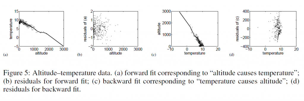
Then, they too consider temperature and altitude pairings.

tempaltHere, the correct model – altitude causes temperature – results in a much more random scatter of residuals, than the reverse direction model.

Patrik Hoyer and Aapo Hyvärinen are a couple of names from this Helsinki group of researchers whose papers are interesting to read and review.

One of the early champions of this resurgence of interest in causality works from a department of philosophy – Peter Spirtes. It’s almost as if the discussion of causal theory were relegated to philosophy, to be revitalized by machine learning and Big Data:

The rapid spread of interest in the last three decades in principled methods of search or estimation of causal relations has been driven in part by technological developments, especially the changing nature of modern data collection and storage techniques, and the increases in the processing power and storage capacities of computers. Statistics books from 30 years ago often presented examples with fewer than 10 variables, in domains where some background knowledge was plausible. In contrast, in new domains such as climate research (where satellite data now provide daily quantities of data unthinkable a few decades ago), fMRI brain imaging, and microarray measurements of gene expression, the number of variables can range into the tens of thousands, and there is often limited background knowledge to reduce the space of alternative causal hypotheses. Even when experimental interventions are possible, performing the many thousands of experiments that would be required to discover causal relationships between thousands or tens of thousands of variables is often not practical. In such domains, non-automated causal discovery techniques from sample data, or sample data together with a limited number of experiments, appears to be hopeless, while the availability of computers with increased processing power and storage capacity allow for the practical implementation of computationally intensive automated search algorithms over large search spaces.

Introduction to Causal Inference

Granger Causality

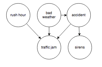
After review, I have come to the conclusion that from a predictive and operational standpoint, causal explanations translate to directed graphs, such as the following:

causegraph

And I think it is interesting the machine learning community focuses on causal explanations for “manipulation” to guide reactive and interactive machines, and that directed graphs (or perhaps a Bayesian networks) are a paramount concept.

Keep that thought, and consider “Granger causality.”

This time series concept is well explicated in C.W.J. Grangers’ 2003 Nobel Prize lecture – which motivates its discovery and links with cointegration.

An earlier concept that I was concerned with was that of causality. As a postdoctoral student in Princeton in 1959–1960, working with Professors John Tukey and Oskar Morgenstern, I was involved with studying something called the “cross-spectrum,” which I will not attempt to explain. Essentially one has a pair of inter-related time series and one would like to know if there are a pair of simple relations, first from the variable X explaining Y and then from the variable Y explaining X. I was having difficulty seeing how to approach this question when I met Dennis Gabor who later won the Nobel Prize in Physics in 1971. He told me to read a paper by the eminent mathematician Norbert Wiener which contained a definition that I might want to consider. It was essentially this definition, somewhat refined and rounded out, that I discussed, together with proposed tests in the mid 1960’s.

The statement about causality has just two components: 1. The cause occurs before the effect; and 2. The cause contains information about the effect that that is unique, and is in no other variable.

A consequence of these statements is that the causal variable can help forecast the effect variable after other data has first been used. Unfortunately, many users concentrated on this forecasting implication rather than on the original definition. At that time, I had little idea that so many people had very fixed ideas about causation, but they did agree that my definition was not “true causation” in their eyes, it was only “Granger causation.” I would ask for a definition of true causation, but no one would reply. However, my definition was pragmatic and any applied researcher with two or more time series could apply it, so I got plenty of citations. Of course, many ridiculous papers appeared.

When the idea of cointegration was developed, over a decade later, it became clear immediately that if a pair of series was cointegrated then at least one of them must cause the other. There seems to be no special reason why there two quite different concepts should be related; it is just the way that the mathematics turned out

In the two-variable case, suppose we have time series Y={y1,y2,…,yt} and X = {x1,..,xt}. Then, there are, at the outset, two cases, depending on whether Y and X are stationary or nonstationary. The classic case is where we have an autoregressive relationship for yt,

yt = a0+a1yt-1+..+akyt-k

and this relationship can be shown to be a weaker predictor than


yt = a0+a1yt-1+..+akyt-k + b0+b1xt-1+..+bmxt-m

In this case, we say that X exhibits Granger causality with respect to Y.

Of course, if Y and X are nonstationary time series, autoregressive predictive equations make no sense, and instead we have the case of cointegration of time series, where in the two-variable case,

yt=φxt-1+ut

and the series of residuals ut are reduced to a white noise process.

So these cases follow what good old Wikipedia says,

A time series X is said to Granger-cause Y if it can be shown, usually through a series of t-tests and F-tests on lagged values of X (and with lagged values of Y also included), that those X values provide statistically significant information about future values of Y.

There are a number of really interesting extensions of this linear case, discussed in a recent survey paper.

Stern points out that the main enemies or barriers to establishing causal relations are endogeneity and omitted variables.

So I find that margin loans and the level of the S&P 500 appear to be mutually interrelated. Thus, it is forecasts of the S&P 500 can be improved with lagged values of margin loans, and you can improve forecasts of the monthly total of margin loans with lagged values of the S&P 500 – at least over broad ranges of time and in the period since 2008. The predictions of the S&P 500 with lagged values of margin loans, however, are marginally more powerful or accurate predictions.

Stern gives a colorful example where an explanatory variable is clearly exogenous and appears to have a significant effect on the dependent variable and yet theory suggests that the relationship is spurious and due to omitted variables that happen to be correlated with the explanatory variable in question.

Westling (2011) regresses national economic growth rates on average reported penis lengths and other variables and finds that there is an inverted U shape relationship between economic growth and penis length from 1960 to 1985. The growth maximizing length was 13.5cm, whereas the global average was 14.5cm. Penis length would seem to be exogenous but the nature of this relationship would have changed over time as the fastest growing region has changed from Europe and its Western Offshoots to Asia. So, it seems that the result is likely due to omitted variables bias.

Here Stern notes that Westling’s data indicates penis length is lowest in Asia and greatest in Africa with Europe and its Western Offshoots having intermediate lengths.

There’s a paper which shows stock prices exhibit Granger causality with respect to economic growth in the US, but vice versa does not obtain. This is a good illustration of the careful ste-by-step in conducting this type of analysis, and how it is in fact fraught with issues of getting the number of lags exactly right and avoiding big specification problems.

Just at the moment when it looks as if the applications of Granger causality are petering out in economics, neuroscience rides to the rescue. I offer you a recent article from a journal in computation biology in this regard – Measuring Granger Causality between Cortical Regions from Voxelwise fMRI BOLD Signals with LASSO.

Here’s the Abstract:

Functional brain network studies using the Blood Oxygen-Level Dependent (BOLD) signal from functional Magnetic Resonance Imaging (fMRI) are becoming increasingly prevalent in research on the neural basis of human cognition. An important problem in functional brain network analysis is to understand directed functional interactions between brain regions during cognitive performance. This problem has important implications for understanding top-down influences from frontal and parietal control regions to visual occipital cortex in visuospatial attention, the goal motivating the present study. A common approach to measuring directed functional interactions between two brain regions is to first create nodal signals by averaging the BOLD signals of all the voxels in each region, and to then measure directed functional interactions between the nodal signals. Another approach, that avoids averaging, is to measure directed functional interactions between all pairwise combinations of voxels in the two regions. Here we employ an alternative approach that avoids the drawbacks of both averaging and pairwise voxel measures. In this approach, we first use the Least Absolute Shrinkage Selection Operator (LASSO) to pre-select voxels for analysis, then compute a Multivariate Vector AutoRegressive (MVAR) model from the time series of the selected voxels, and finally compute summary Granger Causality (GC) statistics from the model to represent directed interregional interactions. We demonstrate the effectiveness of this approach on both simulated and empirical fMRI data. We also show that averaging regional BOLD activity to create a nodal signal may lead to biased GC estimation of directed interregional interactions. The approach presented here makes it feasible to compute GC between brain regions without the need for averaging. Our results suggest that in the analysis of functional brain networks, careful consideration must be given to the way that network nodes and edges are defined because those definitions may have important implications for the validity of the analysis.

So Granger causality is still a vital concept, despite its probably diminishing use in econometrics per se.

Let me close with this thought and promise a future post on the Kaggle and machine learning competitions on identifying the direction of causality in pairs of variables without context.

Correlation does not imply causality—you’ve heard it a thousand times. But causality does imply correlation.

Links – February 1, 2014

IT and Big Data

Kayak and Big Data Kayak is adding prediction of prices of flights over the coming 7 days to its meta search engine for the travel industry.

China’s Lenovo steps into ring against Samsung with Motorola deal Lenovo Group, the Chinese technology company that earns about 80 percent of its revenue from personal computers, is betting it can also be a challenger to Samsung Electronics Co Ltd and Apple Inc in the smartphone market.

5 Things To Know About Cognitive Systems and IBM Watson Rob High video on Watson at http://www.redbooks.ibm.com/redbooks.nsf/pages/watson?Open. Valuable to review. Watson is probably different than you think. Deep natural language processing.

Playing Computer Games and Winning with Artificial Intelligence (Deep Learning) Pesents the first deep learning model to successfully learn control policies directly from high-dimensional sensory input using reinforcement learning. The model is a convolutional neural network, trained with a variant of Q-learning, whose input is raw pixels and whose output is a value function estimating future rewards… [applies] method to seven Atari 2600 games from the Arcade Learning Environment, with no adjustment of the architecture or learning algorithm…outperforms all previous approaches on six of the games and surpasses a human expert on three of them.

Global Economy

China factory output points to Q1 lull Chinese manufacturing activity slipped to its lowest level in six months, with indications of slowing growth for the quarter to come in the world’s second-largest economy.

Japan inflation rises to a 5 year high, output rebounds Japan’s core consumer inflation rose at the fastest pace in more than five years in December and the job market improved, encouraging signs for the Bank of Japan as it seeks to vanquish deflation with aggressive money printing.

Coup Forecasts for 2014

coupforecast                       

World risks deflationary shock as BRICS puncture credit bubbles Ambrose Evans-Pritchard does some nice analysis in this piece.

Former IMF Chief Economist, Now India’s Central Bank Governor Rajan Takes Shot at Bernanke’s Destabilizing Policies

Some of his key points:

Emerging markets were hurt both by the easy money which flowed into their economies and made it easier to forget about the necessary reforms, the necessary fiscal actions that had to be taken, on top of the fact that emerging markets tried to support global growth by huge fiscal and monetary stimulus across the emerging markets. This easy money, which overlaid already strong fiscal stimulus from these countries. The reason emerging markets were unhappy with this easy money is “This is going to make it difficult for us to do the necessary adjustment.” And the industrial countries at this point said, “What do you want us to do, we have weak economies, we’ll do whatever we need to do. Let the money flow.”

Now when they are withdrawing that money, they are saying, “You complained when it went in. Why should you complain when it went out?” And we complain for the same reason when it goes out as when it goes in: it distorts our economies, and the money coming in made it more difficult for us to do the adjustment we need for the sustainable growth and to prepare for the money going out

International monetary cooperation has broken down. Industrial countries have to play a part in restoring that, and they can’t at this point wash their hands off and say we’ll do what we need to and you do the adjustment. ….Fortunately the IMF has stopped giving this as its mantra, but you hear from the industrial countries: We’ll do what we have to do, the markets will adjust and you can decide what you want to do…. We need better cooperation and unfortunately that’s not been forthcoming so far.

Science Perspective

Researchers Discover How Traders Act Like Herds And Cause Market Bubbles

Building on similarities between earthquakes and extreme financial events, we use a self-organized criticality-generating model to study herding and avalanche dynamics in financial markets. We consider a community of interacting investors, distributed in a small-world network, who bet on the bullish (increasing) or bearish (decreasing) behavior of the market which has been specified according to the S&P 500 historical time series. Remarkably, we find that the size of herding-related avalanches in the community can be strongly reduced by the presence of a relatively small percentage of traders, randomly distributed inside the network, who adopt a random investment strategy. Our findings suggest a promising strategy to limit the size of financial bubbles and crashes. We also obtain that the resulting wealth distribution of all traders corresponds to the well-known Pareto power law, while that of random traders is exponential. In other words, for technical traders, the risk of losses is much greater than the probability of gains compared to those of random traders. http://pre.aps.org/abstract/PRE/v88/i6/e062814

Blogs review: Getting rid of the Euler equation – the equation at the core of modern macro The Euler equation is one of the fundamentals, at a deep level, of dynamic stochastic general equilibrium (DSGE) models promoted as the latest and greatest in theoretical macroeconomics. After the general failures in mainstream macroeconomics with 2008-09, DGSE have come into question, and this review is interesting because it suggests, to my way of thinking, that the Euler equation linking past and future consumption patterns is essentially grafted onto empirical data artificially. It is profoundly in synch with neoclassical economic theory of consumer optimization, but cannot be said to be supported by the data in any robust sense. Interesting read with links to further exploration.

BOSTON COLLOQUIUM FOR PHILOSOPHY OF SCIENCE: Revisiting the Foundations of Statistics – check this out – we need the presentations online.

Hal Varian and the “New” Predictive Techniques

Big Data: New Tricks for Econometrics is, for my money, one of the best discussions of techniques like classification and regression trees, random forests, and penalized  regression (such as lasso, lars, and elastic nets) that can be found.

Varian, pictured aove, is emeritus professor in the School of Information, the Haas School of Business, and the Department of Economics at the University of California at Berkeley. Varian retired from full-time appointments at Berkeley to become Chief Economist at Google.

He also is among the elite academics publishing in the area of forecasting according to IDEAS!.

Big Data: New Tricks for Econometrics, as its title suggests, uses the wealth of data now being generated (Google is a good example) as a pretext for promoting techniques that are more well-known in machine learning circles, than in econometrics or standard statistics, at least as understood by economists.

First, the sheer size of the data involved may require more sophisticated 18 data manipulation tools. Second, we may have more potential predictors than appropriate for estimation, so we need to do some kind of variable selection. Third, large data sets may allow for more flexible relationships than simple linear models. Machine learning techniques such as decision trees, support vector machines, neural nets, deep learning and so on may allow for more effective ways to model complex relationships.

He handles the definitional stuff deftly, which is good, since there is not standardization of terms yet in this rapidly evolving field of data science or predictive analytics, whatever you want to call it.

Thus, “NoSQL” databases are

sometimes interpreted as meaning “not only SQL.” NoSQL databases are more primitive than SQL databases in terms of data manipulation capabilities but can handle larger amounts of data.

The essay emphasizes out-of-sample prediction and presents a nice discussion of k-fold cross validation.

1. Divide the data into k roughly equal subsets and label them by s =1; : : : ; k. Start with subset s = 1.

2. Pick a value for the tuning parameter.

3. Fit your model using the k -1 subsets other than subset s.

4. Predict for subset s and measure the associated loss.

5. Stop if s = k, otherwise increment s by 1 and go to step 2.

Common choices for k are 10, 5, and the sample size minus 1 (“leave one out”). After cross validation, you end up with k values of the tuning parameter and the associated loss which you can then examine to choose an appropriate value for the tuning parameter. Even if there is no tuning parameter, it is useful to use cross validation to report goodness-of-t measures since it measures out-of-sample performance which is what is typically of interest.

Varian remarks that Test-train and cross validation, are very commonly used in machine learning and, in my view, should be used much more in economics, particularly when working with large datasets

But this essay is by no means methodological, and presents several nice worked examples, showing how, for example, regression trees can outperform logistic regression in analyzing survivors of the sinking of the Titanic – the luxury ship, and how several of these methods lead to different imputations of significance to the race factor in the Boston Housing Study.

The essay also presents easy and good discussions of bootstrapping, bagging, boosting, and random forests, among the leading examples of “new” techniques – new to economists.

For the statistics wonks, geeks, and enthusiasts among readers, here is a YouTube presentation of the paper cited above with extra detail.