Category Archives: stock market forecasts

anatomy of an asset bubble, asset bubbles, celebrity forecasters, financial forecasts, financial risk management, forecasting asset bubbles, forecasting research, forecasting turning points, stock market forecasts

Didier Sornette – Celebrity Bubble Forecaster

February 6, 2014 Clive Jones

Professor Didier Sornette, who holds the Chair in Entreprenuerial Risks at ETH Zurich, is an important thinker, and it is heartening to learn the American Association for the Advancement of Science (AAAS) is electing Professor Sornette a Fellow.

It is impossible to look at, say, the historical performance of the S&P 500 over the past several decades, without concluding that, at some point, the current surge in the market will collapse, as it has done previously when valuations ramped up so rapidly and so far.

Sornette focuses on asset bubbles and has since 1998, even authoring a book in 2004 on the stock market.

At the same time, I think it is fair to say that he has been largely ignored by mainstream economics (although not finance), perhaps because his training is in physical science. Indeed, many of his publications are in physics journals – which is interesting, but justified because complex systems dynamics cross the boundaries of many subject areas and sciences.

Over the past year or so, I have perused dozens of Sornette papers, many from the extensive list at http://www.er.ethz.ch/publications/finance/bubbles_empirical.

This list is so long and, at times, technical, that videos are welcome.

Along these lines there is Sornette’s Ted talk (see below), and an MP4 file which offers an excellent, high level summary of years of research and findings. This MP4 video was recorded at a talk before the International Center for Mathematical Sciences at the University of Edinburgh.

Intermittent criticality in financial markets: high frequency trading to large-scale bubbles and crashes. You have to download the file to play it.

By way of précis, this presentation offers a high-level summary of the roots of his approach in the economics literature, and highlights the role of a central differential equation for price change in an asset market.

So since I know everyone reading this blog was looking forward to learning about a differential equation, today, let me highlight the importance of the equation,

dp/dt = cp^d

This basically says that price change in a market over time depends on the level of prices – a feature of markets where speculative forces begin to hold sway.

This looks to be a fairly simple equation, but the solutions vary, depending on the values of the parameters c and d. For example, when c>0 and the exponent d is greater than one, prices change faster than exponentially and within some finite period, a singularity is indicated by the solution to the equation. Technically, in the language of differential equations this is called a finite time singularity.

Well, the essence of Sornette’s predictive approach is to estimate the parameters of a price equation that derives, ultimately, from this differential equation in order to predict when an asset market will reach its peak price and then collapse rapidly to lower prices.

The many sources of positive feedback in asset pricing markets are the basis for the faster than exponential growth, resulting from d>1. Lots of empirical evidence backs up the plausibility and credibility of herd and imitative behaviors, and models trace out the interaction of prices with traders motivated by market fundamentals and momentum traders or trend followers.

Interesting new research on this topic shows that random trades could moderate the rush towards collapse in asset markets – possibly offering an alternative to standard regulation.

The important thing, in my opinion, is to discard notions of market efficiency which, even today among some researchers, result in scoffing at the concept of asset bubbles and basic sabotage of research that can help understand the associated dynamics.

Here is a TED talk by Sornette from last summer.

anatomy of an asset bubble, ARIMA models, asset bubbles, financial forecasting, financial forecasts, stock market forecasts

Simulating the SPDR SPY Index

February 5, 2014 Clive Jones

Here is a simulation of the SPDR SPY exchange traded fund index, using an autoregressive model estimated with maximum likehood methods, assuming the underlying distribution is not normal, but is instead a Student t distribution.

The underlying model is of the form

SPYRR_t=a₀+a₁SPYRR_t-1…a₃₀SPYRR_t-30

Where SPYRR is the daily return (trading day to trading day) of the SPY, based on closing prices.

This is a linear model, and an earlier post lists its exact parameters or, in other words, the coefficients attached to each of the lagged terms, as well as the value of the constant term.

This model is estimated on a training sample of daily returns from 1993 to 2008, and, is applied to out-of-sample data from 2008 to the present. It predicts about 53 percent of the signs of the next-day-returns correctly. The model generates more profits in the 2008 to the present period than a Buy & Hold strategy.

The simulation listed above uses the model equation and parameters, generating a series of 4000 values recursively, adding in randomized error terms from the fit of the equation to the training or estimation data.

This is work-in-progress. Currently, I am thinking about how to properly incorporate volatility. Obviously, any number of realizations are possible. The chart shows one of them, which has an uncanny resemblance to the actual historical series, due to the fact that volatility is created over certain parts of the simulation, in this case by chance.

To review, I set in motion the following process:

Predict a xt = f(xt-1,..,xt-30) based on the 30 coefficients and a constant term from the autoregressive model, applied to 30 preceding values of xt generated by this process (The estimation is initialized with the first 30 actual values of the test data).
Randomly select a residual for this xt based on the empirical distribution of errors from the fit of the predictive relationship to the training set.
Iterate.

The error distribution looks like this.

This is obviously not a normal distribution, since “too many” predictive errors are concentrated around the zero error line.

For puzzles and problems, this is a fertile area for research, and you can make money. But obviously, be careful.

In any case, I think this research, in an ultimate analysis, converges to the work being done by Didier Sornette and his co-researchers and co-authors. Sornette et al develop an approach through differential equations, focusing on critical points where a phase shift occurs in trading with a rapid collapse of an asset bubble.

This approach comes at similar, semi-periodic, logarithmically increasing values through linear autoregressive equations, which, as is well known, have complex dynamics when analyzed as difference equations.

The prejudice in economics and econometrics that “you can’t predict the stock market” is an impediment to integrating these methods.

While my research on modeling stock prices is a by-product of my general interest in forecasting and quantitative techniques, I may have an advantage because I will try stuff that more seasoned financial analysts may avoid, because they have been told it does not work.

So I maintain it is possible, at least in the era of quantitative easing (QE), to profit from autoregressive models of daily returns on a major index like the SPY. The models are, admittedly, weak predictors, but they interact with the weird error structure of SPY daily returns in interesting ways. And, furthermore, it is possible for anyone to verify my claims simply by calculating the predictions for the test period from 2008 to the present and then looking at what a Buy & Hold Strategy would have done over the same period.

In this post, I reverse the process. I take one of my autoregressive models and generate, by simulation, time series that look like historical SPY daily values.

On Sornette, about which I think we will be hearing more, since currently the US stock market seems to be in correction model, see – Turbulent times ahead: Q&A with economist Didier Sornette. Also check http://www.er.ethz.ch/presentations/index.

financial forecasting, financial forecasts, random walk, stock market forecasts

Predicting the Stock Market, Making Profits in the Stock Market

February 2, 2014 Clive Jones

Often, working with software and electronics engineers, a question comes up – “if you are so good at forecasting (company sales, new product introductions), why don’t you forecast the stock market?” This might seem to be a variant of “if you are so smart, why aren’t you rich?” but I think it usually is asked more out of curiosity, than malice.

In any case, my standard reply has been that basically you could not forecast the stock market; that the stock market was probably more or less a random walk. If it were possible to forecast the stock market, someone would have done it. And the effect of successful forecasts would be to nullify further possibility of forecasting. I own an early edition of Burton Malkiel’s Random Walk Down Wall Street.

Today, I am in the amazing position of earnestly attempting to bring attention to the fact that, at least since 2008, a major measure of the stock market – the SPY ETF which tracks the S&P 500 Index, in fact, can be forecast. Or, more precisely, a forecasting model for daily returns of the SPY can lead to sustainable, increasing returns over the past several years, despite the fact the forecasting model, is, by many criteria, a weak predictor.

I think this has to do with special features of this stock market time series which have not, heretofore, received much attention in econometric modeling.

So here are the returns from applying this SPY from early 2008 to early 2014 (click to enlarge).

I begin with a $1000 investment 1/22/2008 and trade potentially every day, based on either the Trading Program or a Buy & Hold strategy.

Now there are several remarkable things about this Trading Program and the underlying regression model.

First, the regression model is a most unlikely candidate for making money in the stock market. The R²or coefficient of determination is 0.0238, implying that the 60 regressors predict only 2.38 percent of the variation in the SPY rates of return. And it’s possible to go on in this vein – for example, the F-statistic indicating whether there is a relation between the regressors and the dependent variable is 1.42, just marginally above the 1 percent significance level, according to my reading of the Tables.

And the regression with 60 regressors correctly predicts the correct sign of the next days’ SPY rates of return only 50.1 percent of the time.

This, of course, is a key fact, since the Trading Program (see below) is triggered by positive predictions of the next day’s rate of return. When the next day rate of return is predicted to be positive and above a certain minimum value, the Trading Program buys SPY with the money on hand from previous sales – or, if the investor is already holding SPY because the previous day’s prediction also was positive, the investor stands pat.

The Conventional Wisdom

Professor Jim Hamilton, one of the principals (with Menzie Chin) in Econbrowser had a post recently On R-squared and economic prediction which makes the sensible point that R² or the coefficient of determination in a regression is not a great guide to predictive performance. The post shows, among other things, that first differences of the daily S&P 500 index values regressed against lagged values of these first differences have low R² – almost zero.

Hamilton writes,

Actually, there’s a well-known theory of stock prices that claims that an R-squared near zero is exactly what you should find. Specifically, the claim is that everything anybody could have known last month should already have been reflected in the value of pt -1. If you knew last month, when pt-1 was 1800, that this month it was headed to 1900, you should have bought last month. But if enough savvy investors tried to do that, their buy orders would have driven pt-1 up closer to 1900. The stock price should respond the instant somebody gets the news, not wait around a month before changing.

That’s not a bad empirical description of stock prices– nobody can really predict them. If you want a little fancier model, modern finance theory is characterized by the more general view that the product of today’s stock return with some other characteristics of today’s economy (referred to as the “pricing kernel”) should have been impossible to predict based on anything you could have known last month. In this formulation, the theory is confirmed– our understanding of what’s going on is exactly correct– only if when regressing that product on anything known at t – 1 we always obtain an R-squared near zero.

Well, I’m in the position here of seeking to correct one of my intellectual mentors. Although Professor Hamilton and I have never met nor communicated directly, I did work my way through Hamilton’s seminal book on time series analysis – and was duly impressed.

I am coming to the opinion that the success of this fairly low-power regression model on the SPY must have to do with special characteristics of the underlying distribution of rates of return.

For example, it’s interesting that the correlations between the (61) regressors and the daily returns are higher, when the absolute values of the dependent variable rates of return are greater. There is, in fact, a lot of meaningless buzz at very low positive and negative rates of return. This seems consistent with the odd shape of the residuals of the regression, shown below.

I’ve made this point before, most recently in a post-2014 post Predicting the S&P 500 or the SPY Exchange-Traded Fund, where I actually provide coefficients for a autoregressive model estimated by Matlab’s arima procedure. That estimation, incidentally, takes more account of the non-normal characteristics of the distribution of the rates of return, employing a t-distribution in maximum likelihood estimates of the parameters. It also only uses lagged values of SPY daily returns, and does not include any contribution from the VIX.

I guess in the remote possibility Jim Hamilton glances at either of these posts, it might seem comparable to reading claims of a perpetual motion machine, a method to square the circle, or something similar- quackery or wrong-headedness and error.

A colleague with a Harvard Ph.D in applied math, incidentally, has taken the trouble to go over my data and numbers, checking and verifying I am computing what I say I am computing.

Further details follow on this simple ordinary least squares (OLS) regression model I am presenting here.

Data and the Model

The focus of this modeling effort is on the daily returns of the SPDR S&P 500 (SPY), calculated with daily closing prices, as -1+(today’s closing price/the previous trading day’s closing price). The data matrix includes 30 lagged values of the daily returns of the SPY (SPYRR) along with 30 lagged values of the daily returns of the VIX volatility index (VIXRR). The data span from 11/26/1993 to 1/16/2014 – a total of 5,072 daily returns.

There is enough data to create separate training and test samples, which is good, since in-sample performance can be a very poor guide to out-of-sample predictive capabilities. The training sample extends from 11/26/1993 to 1/18/2008, for a total of 3563 observations. The test sample is the complement of this, extending from 1/22/2008 to 1/16/2014, including 1509 cases.

So the basic equation I estimate is of the form

SPYRR_t=a₀+a₁SPYRR_t-1…a₃₀SPYRR_t-30+b₁VIXRR_t-1+..+b30VIXRR_t-30

Thus, the equation has 61 parameters – 60 coefficients multiplying into the lagged returns for the SPY and VIX indices and a constant term.

Estimation Technique

To make this simple, I estimate the above equation with the above data by ordinary least squares, implementing the standard matrix equation b = (X^TX)^-1X^TY, where T indicates ‘transpose.’ I add a leading column of ‘1’s’ to the data matrix X to allow for a constant term a₀. I do not mean center or standardize the observations on daily rates of return.

Rule for Trading Program and Summing UP

The Trading Program is the same one I described in earlier blog posts on this topic. Basically, I update forecasts every day and react to the forecast of the next day’s daily return. If it is positive, and now above a certain minimum, I either buy or hold. If it is not, I sell or do not enter the market. Oh yeah, I start out with $1000 in all these simulations and only trade with proceeds from this initial investment.

The only element of unrealism is that I have to predict the closing price of the SPY some short period before the close of the market to be able to enter my trade. I have not looked closely at this, but I am assuming volatility in the last few seconds is bounded, except perhaps in very unusual circumstances.

I take the trouble to present the results of an OLS regression to highlight the fact that what looks like a weak model in this context can work to achieve profits. I don’t think that point has ever been made. There are, of course, all sorts of possibilities for further optimizing this model.

I also suspect that monetary policy has some role in the success of this Trading Program over this period – so it would be interesting to look at similar models at other times and perhaps in other markets.

ARIMA models, Monte Carlo simulation, predictive analytics, stock market forecasts

Predicting the S&P 500 or the SPY Exchange-Traded Fund

January 12, 2014 Clive Jones 2 Comments

By some lights, predicting the stock market is the ultimate challenge. Tremendous resources are dedicated to it – pundits on TV, specialized trading programs, PhD’s doing high-end quantitative analysis in hedge funds. And then, of course, theories of “rational expectations” and “efficient markets” deny the possibility of any consistent success at stock market prediction, on grounds that stock prices are basically random walks.

I personally have not dabbled much in forecasting the market, until about two months ago, when I grabbed a bunch of data on the S&P 500 and tried some regressions with lags on S&P 500 daily returns and daily returns from the VIX volatility index.

What I discovered is completely replicable, and also, so far as I can see, is not widely known.

An autoregressive time series model of S&P 500 or SPY daily returns, built with data from 1993 to early 2008, can outperform a Buy & Hold strategy initiated with out-of-sample data beginning January 2008 and carrying through to recent days.

Here is a comparison of cumulative gains from a Buy & Hold strategy initiated January 23, 2008 with a Trading Strategy informed by my autoregressive (AR) model.

So, reading this chart, investing $1000 January 23, 2008 and not touching this investment leads to cumulative returns of $1586.84 – that’s the Buy & Hold strategy.

The AR trading model, however, generates cumulative returns over this period of $2097.

The trading program based on the autoregressive model I am presenting here works like this. The AR model predicts the next day return for the SPY, based on the model coefficients (which I detail below) and the daily returns through the current day. So, if there is an element of unrealism, it is because the model is based on the daily returns computed on closing values day-by-day. But, obviously, you have to trade before the closing bell (in standard trading), so you need to use a estimate of the current day’s closing value obtained very close to the bell, before deciding whether to invest, sell, or buy SPY for the next day’s action.

But basically, assuming we can do this, perhaps seconds before the bell, and come close to an estimate of the current day closing price – the AR trading program is to buy SPY if the next day’s return is predicted to be positive – or if you currently hold SPY, to continue holding it. If the next day’s return is predicted to be negative, you sell your holdings.

It’s as simple as that.

So the AR model predicts daily returns on a one-day-ahead basis, using information on daily returns through the current trading day, plus the model coefficients.

Speaking of which, here are the coefficients from the Matlab “printout.”

There are a couple of nuances here. First, these parameter values do not derive from an ordinary least squares (OLS) regression. Instead, they are produced by maximum likelihood estimation, assuming the underlying distribution is a t-distribution (not a Gaussian distribution).

The use of a t-distribution, the idea of which I got to some extent from Nassim Taleb’s new text-in-progress mentioned two posts ago, is motivated by the unusual distribution of residuals of an OLS regression of lagged daily returns.

The proof is in the pudding here, too, since the above coefficients work better than ones developed on the (manifestly incorrect) assumption that the underlying error distribution is Gaussian.

Here is a graph of the 30-day moving averages of the proportion of signs of daily returns correctly predicted by this model.

Overall, about 53 percent of the signs of the daily returns in this out-of-sample period are predicted correctly.

If you look at this graph, too, it’s clear there are some differences in performance over this period. Thus, the accuracy of the model took a dive in 2009, in the depths of the Great Recession. And, model performance achieved significantly higher success proportions in 2012 and early 2013, perhaps related to markets getting used to money being poured in by the Fed’s policies of quantitative easing.

Why This AR Model is Such a Big Deal

I find it surprising that a set of fixed coefficients applied to the past 30 values of the SPY daily returns continue to predict effectively, months and years after the end of the in-sample values.

And, I might add, it’s not clear that updating the AR model always improves the outcomes, although I can do more work on this and also on the optimal sample period generally.

Can this be a matter of pure chance? This has to be considered, but I don’t think so. Monte Carlo simulations of randomized trading indicate that there is a 95 percent chance or better than returns of $2097 in this period are not due to chance. In other words, if I decide to trade on a day based on a flip of a fair coin, heads I buy, tails I sell at the end of the day, it’s highly unlikely I will generate cumulative returns of $2097, given the SPY returns over this period.

The performance of this trading model holds up fairly well through December of last year, but degrades some in the first days of 2014.

I think this is a feather in the cap of forecasting, so to speak. Also, it seems to me that economists promoting ideas of market efficiency and rational expectations need to take these findings into account. Everything is extant. I have provided the coefficients. You can get the SPY daily return values from Yahoo Finance. You can calculate everything yourself to check. I’ve done this several times, slightly differently each time. This time I used Matlab, and its arima estimation procedures work well.

I’m not quite sure what to make of all this, but I think it’s important. Naturally, I am extending these results in my personal model-building, and I can report that extensions are possible. At the same time, no extension of this model I have seen achieves more than nearly 60 percent accuracy in predicting the direction of change or sign of the daily returns, so you are going to lose money sometimes applying these models. Day-trading is a risky business.

asset bubbles, equity premia, Janet Yellen outlook, price earnings ratio, Robert Shiller, stock market forecasts

Stock Market Bubble in 2014?

January 8, 2014 Clive Jones

As of November, Janet Yellen, newly confirmed Chair of the US Federal Reserve Bank, doesn’t think so.

As reported in the Wall Street Journal MONEYBEAT, she said,

“Stock prices have risen pretty robustly”… But looking at several valuation measures — she specifically cited equity-risk premiums — she said: “you would not see stock prices in territory that suggest…bubble-like conditions.”

Her reference to equity-risk premiums sent me to Aswath Damodaran’s webpage, which estimates this metric -basically the extra return investors demand to lure them into stocks and out of the safety of government bonds (in the Updated Data section). It’s definitely an implied value, so it’s hard to judge.

But what are some of the other Pro’s and Con’s regarding a stock market bubble?

Pros – There Definitely is a Bubble

The CAPE (cylically adjusted price earnings ratio) is approaching 2007 levels. This is a metric developed by Robert Shiller and, according to him, is supposed to be a longer term indicator, rather than something that can signal short-term movements in the market. At the same time, recent interviews, who recently shared a Nobel prize in economics, indicate Shiller is currently ‘most worried’ about ‘boom’ in U.S. stock market. Here is his CAPE indext (click this and the other charts here to enlarge).

Several sector and global bubbles are currently reinforcing each other. When one goes pop, it’s likely to bring down the house of cards. In the words of Jesse Columbo, whose warnings in 2007 were prescient,

..the global economic recovery is actually what I call a “Bubblecovery” or a bubble-driven economic recovery that is driven by inflating post-2009 bubbles in China, emerging markets, Australia, Canada, Northern and Western European housing, U.S. housing, U.S. healthcare, U.S. higher education, global bonds, and tech (Web 2.0 and social media).

Margin debt, as reported by the New York Stock Exchange, is also at its all-time highs. Here’s a chart from Advisor Perspectives adjusting margin debt for inflation over a long period.

Con – No Bubble Here

Stocks are the cheapest they have been in decades. This is true, as the chart below shows (based on trailing twelve month “as reported” earnings).

The S&P 500, adjusted for inflation, has not reached the peaks of either 2000 or2007 (chart from All Start Charts)

Bottom Line

I must confess, doing the research for the post, that I think the stock market in the US may have a ways to go, before it hits its peak this time. Dr. Yelen’s appointment suggests quantitative easing (QE) and low interest rates may continue for some time, before the Fed takes away the punch bowl. My guess is that markets are just waiting at this point to see whether this is, in fact, what is likely to happen, or whether others in the Fed will exercise stronger control over policy, now Ben Bernacke is gone.

And, as seems probable, Yellen consolidates her control and signals continuation of current policies, then I suspect we will see some wild increases in asset values here and globally.

asset bubbles, cointegration in time series, financial forecasts, stock market forecasts

What is a Market Bubble?

January 6, 2014 Clive Jones

Let’s ask what might seem to be a silly question, but which turns out to be challenging. What is an asset bubble? How can asset bubbles be identified quantitatively?

Let me highlight two definitions – major in terms of the economics and analytical literature. And remember when working through “definitions” that the last major asset bubbles that burst triggered the recessions of 2008-2009 globally, resulting in the loss of tens of trillions of dollars.

You know, a trillion here and a trillion there, and pretty soon you are talking about real money.

Bubbles as Deviations from Values Linked to Economic Fundamentals

The first is simply that –

An asset price bubble is a price acceleration that cannot be explained in terms of the underlying fundamental economic variables

This comes from Dreger and Zhang, who cite earlier work by Case and Shiller, including their historic paper – Is There A Bubble in the Housing Market (2003)

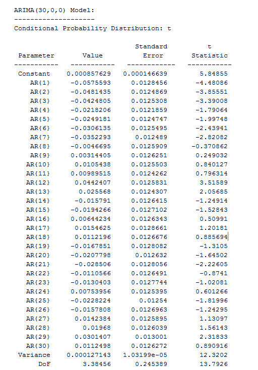
Basically, you need a statistical or an econometric model which “explains” price movements in an asset market. While prices can deviate from forecasts produced by this model on a temporary basis, they will return to the predicted relationship to the set of fundamental variables at some time in the future, or eventually, or in the long run.

The sustained speculative distortions of the asset market then can be measured with reference to benchmark projections with this type of relationship and current values of the “fundamentals.”

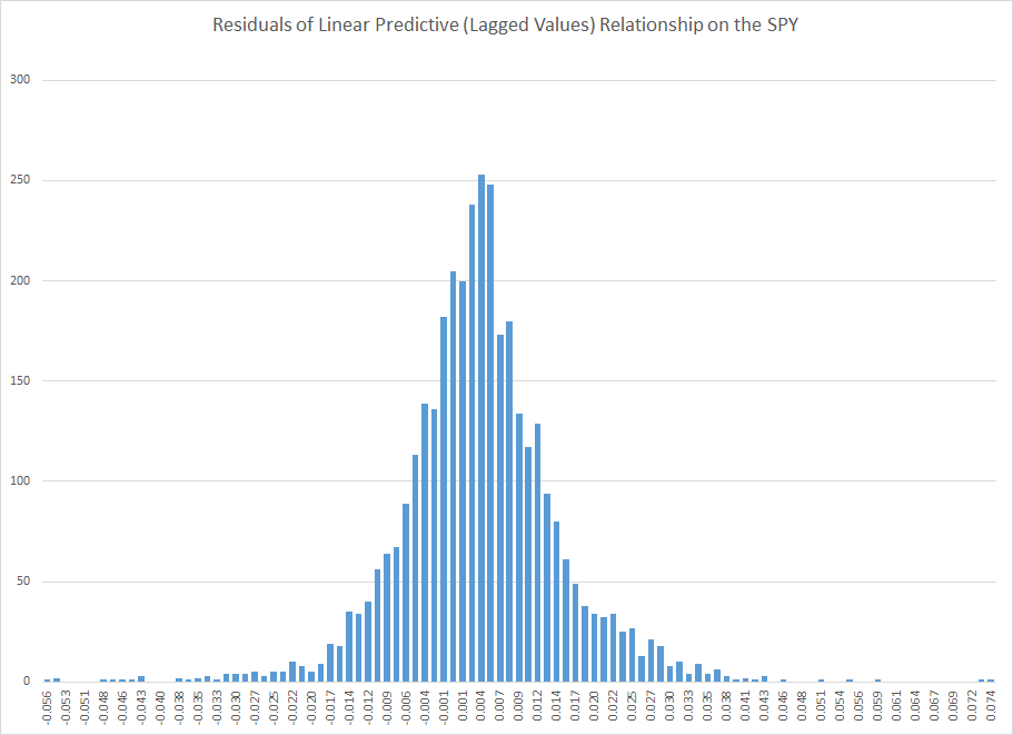
This is the language of co-integrating relationships. The trick, then, is to identify a relationship between the asset price and its fundamental drivers which net out residuals that are white noise, or at least, ARMA – autoregressive moving average – residuals. Good luck with that!

Bubbles as Faster-Than-Exponential Growth

The second definition comes from Didier Sornette and basically is that an asset bubble exists when prices or values are accelerating at a faster-than-exponential rate.

This phenomenon is generated by behaviors of investors and traders that create positive feedback in the valuation of assets and unsustainable growth, leading to a finite-time singularity at some future time… From a technical view point, the positive feedback mechanisms include (i) option hedging, (ii) insurance portfolio strategies, (iii) market makers bid-ask spread in response to past volatility, (iv) learning of business networks and human capital build-up,(v) procyclical financing of firms by banks (boom vs contracting times), (vi) trend following investment strategies, (vii) asymmetric information on hedging strategies viii) the interplay of mark-to-market accounting and regulatory capital requirements. From a behavior viewpoint, positive feedbacks emerge as a result of the propensity of humans to imitate, their social gregariousness and the resulting herding.

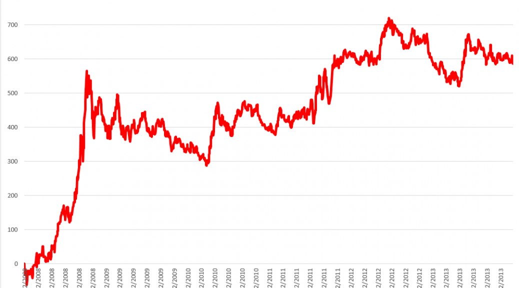
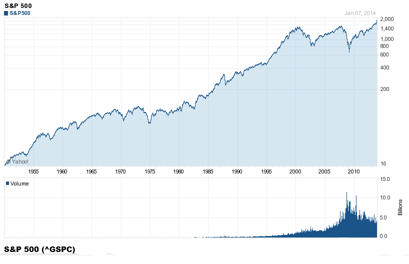
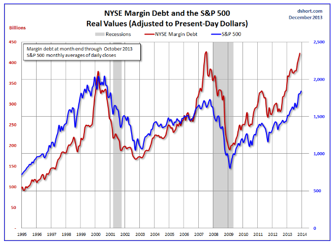
Fundamentals still benchmark asset prices in this approach, as illustrated by this chart.

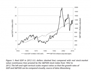
Here GDP and U.S. stock market valuation grow at approximately the same rate, suggesting a “cointegrated relationship,” such as suggested with the first definition of a bubble introduced above.

However, the market has shown three multiple-year periods of excessive valuation, followed by periods of consolidation.

These periods of bubbly growth in prices are triggered by expectations of higher prices and the ability to speculate, and are given precise mathematical expression in the JLS (Johansen-Ledoit-Sornette) model.

The behavioral underpinnings are familiar and can explained with reference to housing, as follows.

The term “bubble” refers to a situation in which excessive future expectations cause prices to rise. For instance, during a house-price bubble, buyers think that a home that they would normally consider too expensive is now an acceptable purchase because they will be compensated by significant further \price increases. They will not need to save as much as they otherwise might, because they expect the increased value of their home to do the saving for them. First-time homebuyers may also worry during a bubble that if they do not buy now, they will not be able to afford a home later. Furthermore, the expectation of large price increases may have a strong impact on demand if people think that home prices are very unlikely to fall, and certainly not likely to fall for long, so that there is little perceived risk associated with an investment in a home.

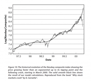
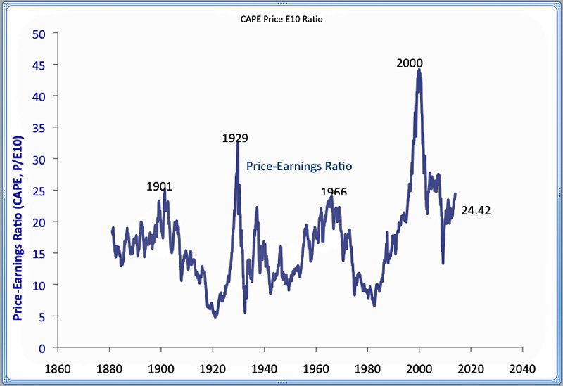
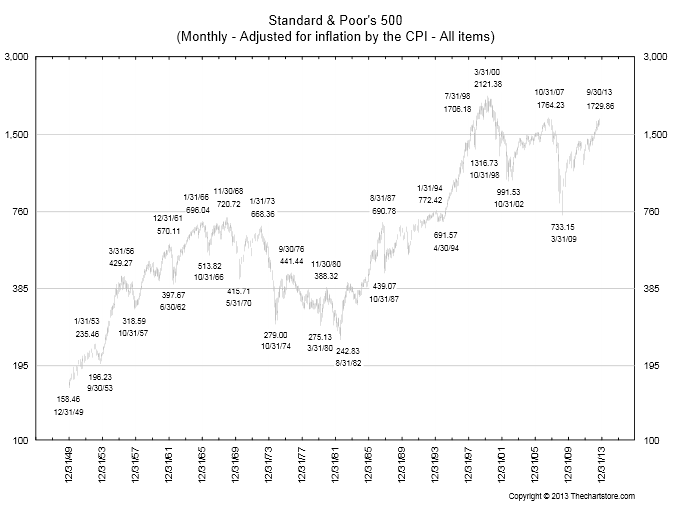
The concept of “faster-than-exponential” growth also is explicated in this chart from a recent article (2011), and originally from Why Stock Markets Crash, published by Princeton.

In a recent methodological piece, Sornette and co-authors cite an extensive list of applications of their approach.

..the JLS model has been used widely to detect bubbles and crashes ex-ante (i.e., with advanced documented notice in real time) in various kinds of markets such as the 2006-2008 oil bubble [5], the Chinese index bubble in 2009 [6], the real estate market in Las Vegas [7], the U.K. and U.S. real estate bubbles [8, 9], the Nikkei index anti-bubble in 1990-1998 [10] and the S&P 500 index anti-bubble in 2000-2003 [11]. Other recent ex-post studies include the Dow Jones Industrial Average historical bubbles [12], the corporate bond spreads [13], the Polish stock market bubble [14], the western stock markets [15], the Brazilian real (R$) – US dollar (USD) exchange rate [16], the 2000-2010 world major stock indices [17], the South African stock market bubble [18] and the US repurchase agreements market [19].

I refer readers to the above link for the specifics of these references. Note, in general, most citations in this post are available as PDF files from a webpage maintained by the Swiss Federal Institute of Technology.

The Psychology of Asset Bubbles

After wrestling with this literature for several months, including some advanced math and econometrics, it seems to me that it all comes down, in the heat of the moment just before the bubble crashes, to psychology.

How does that go?

A recent paper coauthored by Sornette and Cauwels and others summarize the group psychology behind asset bubbles.

In its microeconomic formulation, the model assumes a hierarchical organization of the market, comprised of two groups of agents: a group with rational expectations (the value investors), and a group of “noise” agents, who are boundedly rational and exhibit herding behavior (the trend followers). Herding is assumed to be self-reinforcing, corresponding to a nonlinear trend following behavior, which creates price-to-price positive feedback loops that yield an accelerated growth process. The tension and competition between the rational agents and the noise traders produces deviations around the growing prices that take the form of low-frequency oscillations, which increase in frequency due to the acceleration of the price and the nonlinear feedback mechanisms, as the time of the crash approaches.

Examples of how “irrational” agents might proceed to fuel an asset bubble are given in a selective review of the asset bubble literature developed recently by Anna Scherbina from which I take several extracts below.

For example, there is “feedback trading” involving traders who react solely to past price movements (momentum traders?). Scherbina writes,

In response to positive news, an asset experiences a high initial return. This is noticed by a group of feedback traders who assume that the high return will continue and, therefore, buy the asset, pushing prices above fundamentals. The further price increase attracts additional feedback traders, who also buy the asset and push prices even higher, thereby attracting subsequent feedback traders, and so on. The price will keep rising as long as more capital is being invested. Once the rate of new capital inflow slows down, so does the rate of price growth; at this point, capital might start flowing out, causing the bubble to deflate.

Other mechanisms are biased self-attribution and the representativeness heuristic. In biased self-attribution,

..people to take into account signals that confirm their beliefs and dismiss as noise signals that contradict their beliefs…. Investors form their initial beliefs by receiving a noisy private signal about the value of a security.. for example, by researching the security. Subsequently, investors receive a noisy public signal…..[can be] assumed to be almost pure noise and therefore should be ignored. However, since investors suffer from biased self-attribution, they grow overconfident in their belief after the public signal confirms their private information and further revise their valuation in the direction of their private signal. When the public signal contradicts the investors’ private information, it is appropriately ignored and the price remains unchanged. Therefore, public signals, in expectation, lead to price movements in the same direction as the initial price response to the private signal. These subsequent price moves are not justified by fundamentals and represent a bubble. The bubble starts to deflate after the accumulated public signals force investors to eventually grow less confident in their private signal.

Scherbina describes the representativeness heuristic as follows.

The fourth model combines two behavioral phenomena, the representativeness heuristic and the conservatism bias. Both phenomena were previously documented in psychology and represent deviations from optimal Bayesian information processing. The representativeness heuristic leads investors to put too much weight on attention-grabbing (“strong”) news, which causes overreaction. In contrast, conservatism bias captures investors’ tendency to be too slow to revise their models, such that they underweight relevant but non-attention-grabbing (routine) evidence, which causes underreaction… In this setting, a positive bubble will arise purely by chance, for example, if a series of unexpected good outcomes have occurred, causing investors to over-extrapolate from the past trend. Investors make a mistake by ignoring the low unconditional probability that any company can grow or shrink for long periods of time. The mispricing will persist until an accumulation of signals forces investors to switch from the trending to the mean-reverting model of earnings.

Interesting, several of these “irrationalities” can generate negative, as well as positive bubbles.

Finally, Scherbina makes an important admission, namely that

The behavioral view of bubbles finds support in experimental studies. These studies set up artificial markets with finitely-lived assets and observe that price bubbles arise frequently. The presence of bubbles is often attributed to the lack of common knowledge of rationality among traders. Traders expect bubbles to arise because they believe that other traders may be irrational. Consequently, optimistic media stories and analyst reports may help create bubbles not because investors believe these views but because the optimistic stories may indicate the existence of other investors who do, destroying the common knowledge of rationality.

And let me pin that down further here.

Asset Bubbles – the Evidence From Experimental Economics

Vernon Smith is a pioneer in experimental economics. One of his most famous experiments concerns the genesis of asset bubbles.

Here is a short video about this widely replicated experiment.

Stefan Palan recently surveyed these experiments, and also has a downloadable working paper (2013) which collates data from them.

This article is based on the results of 33 published articles and 25 working papers using the experimental asset market design introduced by Smith, Suchanek and Williams (1988). It discusses the design of a baseline market and goes on to present a database of close to 1600 individual bubble measure observations from experiments in the literature, which may serve as a reference resource for the quantitative comparison of existing and future findings.

A typical pattern of asset bubble formation emerges in these experiments.

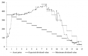
As Smith relates in the video, the experimental market is comprised of student subjects who can both buy and sell and asset which declines in value to zero over a fixed period. Students can earn real money at this, and cannot communicate with others in the experiment.

Noahpinion has further discussion of this type of bubble experiment, which, as Palan writes, is the best-documented experimental asset market design in existence and thus offers a superior base of comparison for new work.

There are convergent lines of evidence about the reality and dynamics of asset bubbles, and a growing appreciation that, empirically, asset bubbles share a number of characteristics.

That may not be enough to convince the mainstream economics profession, however, as a humorous piece by Hirshleifer (2001), quoted by a German researcher a few years back, suggests –

In the muddled days before the rise of modern finance, some otherwise-reputable economists, such as Adam Smith, Irving Fisher, John Maynard Keynes, and Harry Markowitz, thought that individual psychology affects prices. What if the creators of asset pricing theory had followed this thread? Picture a school of sociologists at the University of Chicago proposing the Deficient Markets Hypothesis: that prices inaccurately reflect all available information. A brilliant Stanford psychologist, call him Bill Blunte, invents the Deranged Anticipation and Perception Model (or DAPM), in which proxies for market misevaluation are used to predict security returns. Imagine the euphoria when researchers discovered that these mispricing proxies (such as book/market, earnings/price, and past returns) and mood indicators such as amount of sunlight, turned out to be strong predictors of future returns. At this point, it would seem that the deficient markets hypothesis was the best-confirmed theory in the social sciences.

Business Forecasting