
I’ve posted on ridge regression and the LASSO (Least Absolute Shrinkage and Selection Operator) some weeks back.
Here I want to compare them in connection with variable selection where there are more predictors than observations (“many predictors”).
1. Ridge regression does not really select variables in the many predictors situation. Rather, ridge regression “shrinks” all predictor coefficient estimates toward zero, based on the size of the tuning parameter λ. When ordinary least squares (OLS) estimates have high variability, ridge regression estimates of the betas may, in fact, produce lower mean square error (MSE) in prediction.
2. The LASSO, on the other hand, handles estimation in the many predictors framework and performs variable selection. Thus, the LASSO can produce sparse, simpler, more interpretable models than ridge regression, although neither dominates in terms of predictive performance. Both ridge regression and the LASSO can outperform OLS regression in some predictive situations – exploiting the tradeoff between variance and bias in the mean square error.
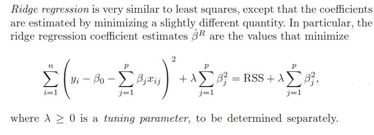
3. Ridge regression and the LASSO both involve penalizing OLS estimates of the betas. How they impose these penalties explains why the LASSO can “zero” out coefficient estimates, while ridge regression just keeps making them smaller. From
An Introduction to Statistical Learning
Similarly, the objective function for the LASSO procedure is outlined by An Introduction to Statistical Learning, as follows

4. Both ridge regression and the LASSO, by imposing a penalty on the regression sum of squares (RWW) shrink the size of the estimated betas. The LASSO, however, can zero out some betas, since it tends to shrink the betas by fixed amounts, as λ increases (up to the zero lower bound). Ridge regression, on the other hand, tends to shrink everything proportionally.
5.The tuning parameter λ in ridge regression and the LASSO usually is determined by cross-validation. Here are a couple of useful slides from Ryan Tibshirani’s Spring 2013 Data Mining course at Carnegie Mellon.


6.There are R programs which estimate ridge regression and lasso models and perform cross validation, recommended by these statisticians from Stanford and Carnegie Mellon. In particular, see glmnet at CRAN. Mathworks MatLab also has routines to do ridge regression and estimate elastic net models.
Here, for example, is R code to estimate the LASSO.
lasso.mod=glmnet(x[train,],y[train],alpha=1,lambda=grid)
plot(lasso.mod)
set.seed(1)
cv.out=cv.glmnet(x[train,],y[train],alpha=1)
plot(cv.out)
bestlam=cv.out$lambda.min
lasso.pred=predict(lasso.mod,s=bestlam,newx=x[test,])
mean((lasso.pred-y.test)^2)
out=glmnet(x,y,alpha=1,lambda=grid)
lasso.coef=predict(out,type=”coefficients”,s=bestlam)[1:20,]
lasso.coef
lasso.coef[lasso.coef!=0]
What You Get
I’ve estimated quite a number of ridge regression and LASSO models, some with simulated data where you know the answers (see the earlier posts cited initially here) and other models with real data, especially medical or health data.
As a general rule of thumb, An Introduction to Statistical Learning notes,
..one might expect the lasso to perform better in a setting where a relatively small number of predictors have substantial coefficients, and the remaining predictors have coefficients that are very small or that equal zero. Ridge regression will perform better when the response is a function of many predictors, all with coefficients of roughly equal size.
The R program glmnet linked above is very flexible, and can accommodate logistic regression, as well as regression with continuous, real-valued dependent variables ranging from negative to positive infinity.
Dear Respectable Mr. or Mrs.,
I’m research assistant Emre DÜNDER, Department of Statistics, Samsun Ondokuz Mayıs University. I have read your blog about lasso regression Your blog is very instructive, thanks a lot. I’m requesting you to give me some information. I performed some simulations for tuning parameter selection based on BIC value. I have seen an interesting result: although the obtained BIC value is small, prediction error is high. I mean, lower BIC valued models correspond to having higher prediction error models. As in your article, BIC selects the models with lower prediction error. Due to I’m familiar with R, I wrote some R codes.
In fact, I saw that, as the selected lambda values increase, prediction error increases. As I saw, BIC tends to select higher lambda values, so this occurs the increment of the prediction error. But in many articles, BIC shows better performance in terms of prediction error. I computed the prediction error as mean((y-yhat)^2).
Why do I obtain such a result? I appreciate if you help me about it. This is a very big conflict. I use R project and I’m sending you some R codes below. I’m waiting for your kind responses.
Best regards.
########################################################################
########################################################################
############################## CODES ###################################
########################################################################
########################################################################
library(mpath)
##### Data Simulation
n<-100
p<-8
x <- scale(matrix(rnorm(n*p),n,p))
beta<-c(3,1.5,5,0,0,0,0,0)
y<-scale(x%*%beta+rnorm(n))
x<-(x-mean(x))/sd(x) #### Normalize x
y<-(y-mean(y))/sd(y) #### Normalize y
v<-data.frame(x,y)
#### BIC Computation
BIC.lasso<-function(x,y,lam){
m <-glmreg(y~x,data=v,family="gaussian",lambda=lam)
kat<-as.matrix(coef(m))[-1]
K<-length(kat[kat!=0])
fit<-coef(m)[1]+x%*%coef(m)[-1]
result<-log(sum((y-fit)^2)/n)+(log(n)*K/n)
return(result)
}
#### Lambda Grids
l<-0:99
lam<-10^(-2+4*l/99)
b<-c();
#### BIC values for every lambda
for(i in 1:100)
b[i]<-BIC.lasso(x,y,lam[i])
min.lam<-lam[which(b==min(b))[1]] ##### First minimum lamda value
plot(lam,b) ######
b #### BIC values vector
##### Comparison of the Methods
l<-cv.glmreg(y~x,family="gaussian",data=v)$lambda.optim
mg<-glmreg(y~x,data=v,family="gaussian",lambda=l)
opt<-glmreg(y~x,data=v,family="gaussian",lambda=min.lam)
cbind(as.matrix(coef(mg)),as.matrix(coef(opt))) ####### BIC shrinks too much
#### Prediction Error Computation
MSE<-function(x,y,lam){
v<-data.frame(x,y)
m<-glmreg(y~x,data=v,family="gaussian",lambda=lam)
fit<-coef(m)[1]+x%*%coef(m)[-1]
mte=apply((y-fit)^2,2,mean)
return(mte)
}
#### Inconsistency ???
BIC.lasso(x,y,l)
BIC.lasso(x,y,min.lam)
MSE(x,y,l)
MSE(x,y,min.lam)
Emre, Thank you for your question – a good one.
A couple of comments.
My understanding is that lasso models usually are selected with CV or cross-validation. Employing a Bayesian Information Critereon (BIC) is a nuance, but there may be tricky stuff in calculating it (see http://stackoverflow.com/questions/27128989/bic-to-choose-lambda-in-lasso-regression).
I would suggestion Cross Validated (for example http://stats.stackexchange.com/questions/25817/is-it-possible-to-calculate-aic-and-bic-for-lasso-regression-models). Hope this helps.