Measuring the Intelligence of Crowds

Researchers at Microsoft Research in the UK and Cambridge University report some fascinating and potentially useful results on crowdsourcing, based on a study of aggregating questions from a standard IQ test on Amazon’s Mechanical Turk (AMT).

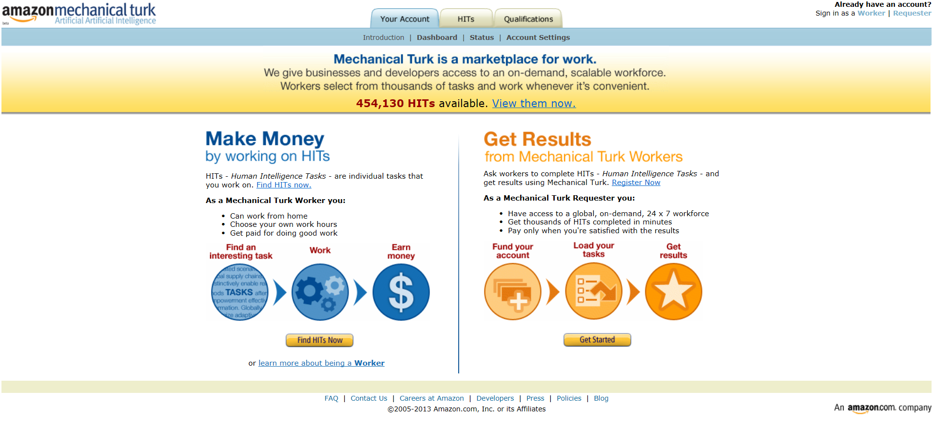
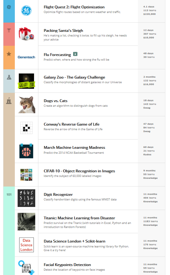
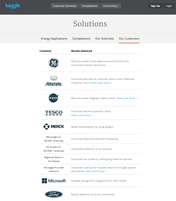
The AMT site provides a place where workers can find problems that requesters have set up for crowdsourcing.

The introductory page to the site looks like this (click to enlarge).

AMT

So here’s an interesting way for people to make some money working from home, at their own hours, and yet stay busy. I’d like to look more deeply into this in a future post, but what these Crowd IQ researchers did is divvy up the questions from a widely utilized IQ test on the AMT site. They studied the effects of changing several parameters on their measures of Crowd IQ, but basically found that, with five or more reputable workers in a group, the Crowd IQ was usually higher than that of the individual workers in the group.

The Abstract for their 2012 study Crowd IQ: Measuring the Intelligence of Crowdsourcing Platforms describes the research and findings succinctly:

We measure crowdsourcing performance based on a standard IQ questionnaire, and examine Amazon’s Mechanical Turk (AMT) performance under different conditions. These include variations of the payment amount offered, the way incorrect responses affect workers’ reputations, threshold reputation scores of participating AMT workers, and the number of workers per task. We show that crowds composed of workers of high reputation achieve higher performance than low reputation crowds, and the effect of the amount of payment is non-monotone—both paying too much and too little affects performance. Furthermore, higher performance is achieved when the task is designed such that incorrect responses can decrease workers’ reputation scores. Using majority vote to aggregate multiple responses to the same task can significantly improve performance, which can be further boosted by dynamically allocating workers to tasks in order to break ties.

The IQ test is Raven’s Standard Progressive Matrices (SPM). If you want to take the test, look here.

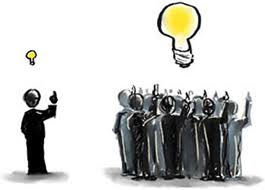
SPM is a nonverbal, multiple-choice intelligence test based on the theory of general ability. The general setup is as in the following example.

Ravenex

Free riders are an interesting problem in a site like the Mechanical Turk. So, if people get paid by the number of correct answers, some simply select responses at random to maximize the speed at which they can put up answers. Because of this, AMT has a reputation mechanism indicating the expected quality of work of a worker, based on his or her past performance.

This research is has real-world implications. For example, increasing the payment for tasks too much results in actually diminuishing the quality of the answers, for a variety of reasons the authors consider.

The “workers” in this AMT-based study did not consult with each other about the answers, but were grouped into teams somehow by the researchers.

Here is a chart showing the increase in crowd IQ with the number of people in the group.

MSFTcurve

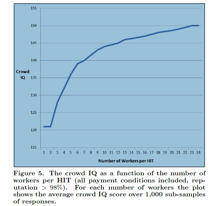
Here a HIT refers to a Human Intelligence Task.

 Recommendations

First, experiment and monitor the performance. Our results suggest that relatively small changes to the parameters of the task may result in great changes in crowd performance. Changing parameters of the task (e.g. reward, time limits, reputation rage) and observing changes in performance may allow you to greatly increase performance. Second, make sure to threaten workers’ reputation by emphasizing that their solutions will be monitored and wrong responses rejected. Obviously, in a real-world setting it may be hard to detect free-riders without using a “gold-set” of test questions to which the requester already knows the correct response. However, designing and communicating HIT rejection conditions can discourage free riding or make it risky and more difficult. For instance, in the case of translation tasks requesters should determine what is not acceptable (e.g. using Google Translate) and may suggest that the response quality would be monitored and solutions of low quality would be rejected. Third, do not over-pay. Although the reward structure obviously depends on the task at hand and the expected amount of effort required to solve it, our results suggest that pricing affects not only the ability to s source enough workers to perform the task but also the quality of the obtained results. Higher rewards are likely to encourage a free-riding behavior and may affect the cognitive abilities of workers by increasing psychological pressure. Thus, for long term projects or tasks that are run repeatedly in a production environment, we believe it is worthwhile to experiment with the reward scheme in order to
find an optimum reward level. Fourth, aggregate multiple solutions to each HIT, preferably using an adaptive sourcing scheme. Even the simplest aggregation method – majority voting – has a potential to greatly improve the quality of the solution. In the context of more complicated tasks, e.g. translations, requesters may consider a two-stage design in which they first request several solutions, and then use another batch of workers to vote for the best one. Additionally, requesters may consider inspecting the responses provided by individuals that often disagree with the crowd – they might be coveted geniuses or free-riders deserving rejection.

Interesting stuff, and makes you want to try crowdsourcing.

Crime Prediction

PredPol markets a crime prediction system tested in and currently used by Los Angeles, CA and Seattle, WA, and under evaluation elsewhere (London, UK). The product takes historic statistics and generates real-time predictions of where new crimes are likely to occur – within highly localized areas.

The spec sheet calls it “cloud-based, easy-to-use” software, offering this basic description.

PredPolsheet1

This has generated lots of press and TV coverage.

In July 2013, there was a thoughtful article in the Economist Don’t even think about it and a piece on National Public Radio (NPR).

A YouTube video features a contribution from one of the company founders – Jeffrey Brantingham.

From what I glean, PredPol takes the idea of crime hotspots a step further, identifying behavioral patterns in burglaries and other property crimes – such as the higher probability of a repeat break-in, or increased probability of a break-in to a neighbor of a house that has been burglarized. Transportation access to and egress from crime sites is also important to criminals – the easier, the better.

The proof is in the pudding. And there have been reductions in property crime in locales where the PredPol system is being applied, although not necessarily increases in arrests. The rationale is that sending additional patrols into the targeted areas deters criminals.

Maybe some of these would-be criminals go elsewhere to rob and steal, but others may simply be deterred, given the criminal mind is at least partly motivated by sheer laziness.

Criticism of PredPol

I can think of several potential flaws.

  • Analytically, there have to be dynamic effects from the success of PredPol in any locale. If successful, in other words, the algorithm will change the crime pattern, and then what?
  • Also, there is a risk of sort of fooling oneself, if the lower crime stats are taken as evidence that the software is effective. Maybe crimes would have decreased anyway.
  • And there are constitutional issues, if police simply stop people to prevent their committing a crime before it has happened, based on the predictions of the software.

Last November, some of the first critical articles about PredPol came out, motivated in part by a SFWeekly article All Tomorrow’s Crimes: The Future of Policing Looks a Lot Like Good Branding

In the meantime, PredPol seems destined for wide application in larger urban areas, and is surely has some of the best PR of any implementation of Big Data and predictive analytics.

Boosting Time Series

If you learned your statistical technique more than ten years ago, consider it necessary to learn a whole bunch of new methods. Boosting is certainly one of these.

Let me pick a leading edge of this literature here – boosting time series predictions.

Results

Let’s go directly to the performance improvements.

In Boosting multi-step autoregressive forecasts, (Souhaib Ben Taieb and Rob J Hyndman, International Conference on Machine Learning (ICML) 2014) we find the following Table applying boosted time series forecasts to two forecasting competition datasets –

HyndmanTable1

The three columns refer to three methods for generating forecasts over horizons of 1-18 periods (M3 Competition and 1-56 period (Neural Network Competition). The column labeled BOOST is, as its name suggests, the error metric for a boosted time series prediction. Either by the lowest symmetric mean absolute percentage error or a rank criterion, BOOST usually outperforms forecasts produced recursively from an autoregressive (AR) model, or forecasts from an AR model directly mapped onto the different forecast horizons.

There were a lot of empirical time series involved in these two datasets –

The M3 competition dataset consists of 3003 monthly, quarterly, and annual time series. The time series of the M3 competition have a variety of features. Some have a seasonal component, some possess a trend, and some are just fluctuating around some level. The length of the time series ranges between 14 and 126. We have considered time series with a range of lengths between T = 117 and T = 126. So, the number of considered time series turns out to be M = 339. For these time series, the competition required forecasts for the next H = 18 months, using the given historical data. The NN5 competition dataset comprises M = 111 time series representing roughly two years of daily cash withdrawals (T = 735 observations) at ATM machines at one of the various cities in the UK. For each time series, the  competition required to forecast the values of the next H = 56 days (8 weeks), using the given historical data.

This research, notice of which can be downloaded from Rob Hyndman’s site, builds on the methodology of Ben Taieb and Hyndman’s recent paper in the International Journal of Forecasting A gradient boosting approach to the Kaggle load forecasting competition. Ben Taieb and Hyndman’s submission came in 5th out of 105 participating teams in this Kaggle electric load forecasting competition, and used boosting algorithms.

Let me mention a third application of boosting to time series, this one from Germany. So we have Robinzonov, Tutz, and Hothorn’s Boosting Techniques for Nonlinear Time Series Models (Technical Report Number 075, 2010 Department of Statistics University of Munich) which focuses on several synthetic time series and predictions of German industrial production.

Again, boosted time series models comes out well in comparisons.

GErmanIndustrialProd

GLMBoost or GAMBoost are quite competitive at these three forecast horizons for German industrial production.

What is Boosting?

My presentation here is a little “black box” in exposition, because boosting is, indeed, mathematically intricate, although it can be explained fairly easily at a very general level.

Weak predictors and weak learners play an important role in bagging and boosting –techniques which are only now making their way into forecasting and business analytics, although the machine learning community has been discussing them for more than two decades.

Machine learning must be a fascinating field. For example, analysts can formulate really general problems –

In an early paper, Kearns and Valiant proposed the notion of a weak learning algorithm which need only achieve some error rate bounded away from 1/2 and posed the question of whether weak and strong learning are equivalent for efficient (polynomial time) learning algorithms.

So we get the “definition” of boosting in general terms:

Boosting algorithms are procedures that “boost” low-accuracy weak learning algorithms to achieve arbitrarily high accuracy.

And a weak learner is a learning method that achieves only slightly better than chance correct classification of binary outcomes or labeling.

This sounds like the best thing since sliced bread.

But there’s more.

For example, boosting can be understood as a functional gradient descent algorithm.

Now I need to mention that some of the most spectacular achievements in boosting come in classification. A key text is the recent book Boosting: Foundations and Algorithms (Adaptive Computation and Machine Learning series) by Robert E. Schapire and Yoav Freund. This is a very readable book focusing on AdaBoost, one of the early methods and its extensions. The book can be read on Kindle and is starts out –

boostingquote

So worth the twenty bucks or so for the download.

The papers discussed above vis a vis boosting time series apply p-splines in an effort to estimate nonlinear effects in time series. This is really unfamiliar to most of us in the conventional econometrics and forecasting communities, so we have to start conceptualizing stuff like “knots” and component-wise fitting algortihms.

Fortunately, there is a canned package for doing a lot of the grunt work in R, called mboost.

Bottom line, I really don’t think time series analysis will ever be the same.

Analytics 2013 Conference in Florida

Looking for case studies of data analytics or predictive analytics, or for Big Data applications?

You can hardly do better, on a first cut, than peruse the material now available from October’s Analytics 2013 Conference, held at the Hyatt Regency Hotel in Orlando, Florida.

Presented by SAS, dozens of presentations and posters from the Conference can be downloaded as zip files, unbundling as PDF files.

Download the conference presentations and poster presentations (.zip)

I also took an hour to look at the Keynote Presentation of Dr. Sven Crone of Lancaster University in the UK, now available on YouTube.

Crone, who also is affiliated with the Lancaster Centre for Forecasting, gave a Keynote which was, in places, fascinating, and technical and a little obscure elsewhere – worth watching if you time, or can run it in the background while you sort through your desk, for example.

A couple of slides caught my attention.

One segment gave concrete meaning to the explosion of data available to forecasters and analysts. For example, for electric power load forecasting, it used be the case that you had, perhaps, monthly total loads for the system or several of its parts, or perhaps daily system loads. Now, Crone notes the data to be modeled has increased by orders of magnitude, for example, with Smart Meters recording customer demand at fifteen minute intervals.

 Analytics13A1                      

Another part of Crone’s talk which grabbed my attention was his discussion of forecasting techniques employed by 300 large manufacturing concerns, some apparently multinational in scale. The following graph – which is definitely obscure by virtue of its use of acronyms for types of forecasting systems, like SOP for Sales and Operation Planning – highlights that almost no company uses anything except the simplest methods for forecasting, relying largely on judgmental approaches. This aligns with a survey I once did which found almost no utilities used anything except the simplest per capita forecasting approaches. Perhaps things have changed now.

Analytics13A1 Analytics13A2

Crone suggests relying strictly on judgment becomes sort of silly in the face of the explosion of information now available to management.

Another theme Crone spins in an amusing, graphic way is that the workhorses of business forecasting, such as exponential smoothing, are really products from many decades ago. He uses funny pics of old business/office environments, asking whether this characterizes your business today.

The analytic meat of the presentation comes with exposition of bagging and boosting, as well as creative uses for k-means clustering in time series analysis.

At which point he descends into a technical wonderland of complexity.

Incidentally, Analytics 2014 is scheduled for Frankfurt, Germany June 4-5 this coming Spring.

Watch here for my follow-on post on boosting time series.

Links January 16, 2014

Economic Outlook

Central Station: January Fed Taper on Track

Federal Reserve officials, including a strong supporter of their easy money policies, have so far brushed off the weak employment report as a blip in an otherwise strengthening economic recovery. This suggests they are likely to stick to their plan to gradually wind down their bond-buying program this year as the recovery picks up momentum…

“True, the December jobs report was disappointing,” said Chicago Fed President Charles Evans, who has been a champion of aggressive central bank efforts to spur stronger economic growth. But, he added, “the recent data on economic activity generally have been encouraging” and “importantly, the labor market has improved.”

He said the tentative plan to reduce the monthly bond buys in $10 billion increments “seems quite reasonable” and “it makes sense to continue that in January.

Atlanta Fed President Dennis Lockhart, a centrist on Fed policies, said Monday the December employment report hadn’t shaken his expectation that the central bank would stick to the taper plan.

Meanwhile two opponents of the bond-buying program, Dallas Fed President Richard Fisher and Philadelphia Fed President Charles Plosser indicated in separate speeches Tuesday they were all for winding it down.

Given that chorus, it appears probable Fed officials will trim their monthly bond purchases to $65 billion from $75 billion at their next policy meeting January 28-29 meeting. Now that tapering is under way, the bar for stopping the process seems quite high.

Big Data

Big Data systems are making a difference in the fight against cancer Open source, distributed computing tools speedup an important processing pipeline for genomics data

Big Data to increase e-tailer profits

As tablet and smartphone usage becomes more widespread, shopping online has become quicker and easier and the speed of delivery has become critical in the online fulfilment race.

The group of researchers, which includes Arne Strauss, Assistant Professor of Operational Research at Warwick Business School, propose an analytic approach that will predict when people want their shopping delivered depending on what delivery prices (or incentives such as discounts or loyalty points) are being quoted for different delivery time slots.

It takes into account accepted orders to date as well as orders that are still expected to come in….

The new approach was tested using real shopping data from a major e-grocer in the UK over a period of six months and generated a four per cent increase in profits on average in a simulation study, outperforming traditional delivery pricing policies.

Big Data and Data Science Books – A Baker’s Dozen – from Analytic Bridge

  1. Big Data: A Revolution That Will Transform How We Live, Work, and T…, by Viktor Mayer-Schonberger and Kenneth Cukier
  2. The Signal and the Noise: Why So Many Predictions Fail-but Some Don’t, by Nate Silver
  3. Predictive Analytics: The Power to Predict Who Will Click, Buy, Lie…, by Eric Siegel
  4. The Human Face of Big Data, by Rick Smolan and Jennifer Erwitt
  5. Data Science for Business: What you need to know about data mining …, by Foster Provost and Tom Fawcett
  6. The Black Swan: The Impact of the Highly Improbable, by Nassim Nicholas Taleb
  7. Competing on Analytics: The New Science of Winning, by Thomas H. Davenport and Jeanne G. Harris
  8. Super Crunchers: Why Thinking-by-Numbers is the New Way to Be Smart, by Ian Ayres
  9. Big Data Marketing: Engage Your Customers More Effectively and Driv…, by Lisa Arthur
  10. Journeys to Data Mining: Experiences from 15 Renowned Researchers, by Mohamed Medhat Gaber (editor)
  11. The Fourth Paradigm: Data-Intensive Scientific Discovery, by T.Hey, S.Tansley, and K.Tolle (editors)
  12. Seven Databases in Seven Weeks: A Guide to Modern Databases and the…, by Eric Redmond and Jim Wilson
  13. Data Mining And Predictive Analysis: Intelligence Gathering And Cri…, by Colleen McCue

Social Media

The History and Evolution of Social Media an Infographic (click to enlarge)

socialmediahistory

If you like this, there are many more infographics focusing on social media at https://www.pinterest.com/JuanCMejiaLlano/social-media-ingles/ – some in Spanish. Also check out Top 10 Infographics of 2013 [Daily Infographic].

Economics

Economics: Science, Craft, or Snake Oil? – nice, but sort of equivocating essay by Dani Rodrik from his new offices at the Princeton Institute for Advanced Studies. Answer – all of the above.

Origin and Importance of the Salesman in US – A piece of US business history and culture. I like this.

World Bank Economic Forecast

The World Bank issued its latest Global Economic Prospects report this week, basically offering up a forecast based on dynamics of (a) moderate increases in growth in the US and Europe (assuming no abrupt, but a gradual taper of QE), and (b) slowing, but stable growth in the developing world at a pace still about double that of the “developed” countries.

The story is, as with other macroeconomic forecasts issued recently by investment banks, that constraints, such as the fiscal drag on growth are being loosened, both in the US and in Europe. With currently low interest rates and continuing excess capacity, this suggests more rapid economic US and EU growth in 2014. Together with the still high average rates of growth in China and elsewhere, this suggests to the World Bank economists, that global growth will quicken in 2014.

Here is a World Bank spokesman with the basic story of the new Global Economic Prospects release.

And here are some of the specific numbers in the report (click to enlarge).

WBforecast

The Evolution of Kaggle

Kaggle is evolving in industry-specific directions, although it still hosts general data and predictive analytics contests.

“We liked to say ‘It’s all about the data,’ but the reality is that you have to understand enough about the domain in order to make a business,” said Anthony Goldbloom, Kaggle’s founder and chief executive. “What a pharmaceutical company thinks a prediction about a chemical’s toxicity is worth is very different from what Clorox thinks shelf space is worth. There is a lot to learn in each area.”

Oil and gas, which for Kaggle means mostly fracking wells in the United States, have well-defined data sets and a clear need to find working wells. While the data used in traditional oil drilling is understood, fracking is a somewhat different process. Variables like how long deep rocks have been cooked in the earth may matter. So does which teams are working the fields, meaning early-stage proprietary knowledge is also in play. That makes it a good field to go into and standardize.

(as reported in http://bits.blogs.nytimes.com/2014/01/01/big-data-shrinks-to-grow/?_r=0)

This December 2013 change of direction pushed out Jeremy Howard, Kaggle’s former Chief Data Scientist, who now says he is,

focusing on building new kinds of software that could better learn about the data it was crunching and offer its human owners insights on any subject.

“A lone wolf data scientist can still apply his knowledge to any industry,” he said. “I’m spending time in areas where I have no industrial knowledge and finding things. I’m going to have to build a company, but first I have to spend time as a lone wolf.”

A year or so ago, the company evolved into a service-provider with the objective of linking companies, top competitors and analytical talent, and the more than 100,000 data scientists who compete on its platform.

So Kaggle now features CUSTOMER SOLUTIONS ahead of COMPETITIONS at the head of its homepage, saying We’re the global leader in solving business challenges through predictive analytics. The homepage also features logos from Facebook GE, MasterCard, and NASA, as well as a link Compete as a data scientist for fortune, fame and fun ».

But a look at the competitions underway currently highlight the fact that just a few pay a prize now.

Kaggleactivecomps

Presumeably, companies looking for answers are now steered into the Kaggle network. The Kaggle Team numbers six analysts with experience in several industries, and the Kaggle Community includes scores of data and predictive analytics whizzes, many with “with multiple Kaggle wins.”

Here is a selection of Kaggle Solutions.

KaggleSolutions

This video gives you a good idea of the current focus of the company.

This is a big development in a way, and supports those who point to the need for industry-specific knowledge and experience to do a good job of data analytics.

The Problem of Many Predictors – Ridge Regression and Kernel Ridge Regression

You might imagine that there is an iron law of ordinary least squares (OLS) regression – the number of observations on the dependent (target) variable and associated explanatory variables must be less than the number of explanatory variables (regressors).

Ridge regression is one way to circumvent this requirement, and to estimate, say, the value of p regression coefficients, when there are N<p training sample observations.

This is very helpful in all sorts of situations.

Instead of viewing many predictors as a variable selection problem (selecting a small enough subset of the p explanatory variables which are the primary drivers), data mining operations can just use all the potential explanatory variables, if the object is primarily predicting the value of the target variable. Note, however, that ridge regression exploits the tradeoff between bias and variance – producing biased coefficient estimates with lower variance than OLS (if, in fact, OLS can be applied).

A nice application was developed by Edward Malthouse some years back. Malthouse used ridge regression for direct marketing scoring models (search and you will find a downloadable PDF). These are targeting models to identify customers for offers, so the response to a mailing is maximized. A nice application, but pre-social media in its emphasis on the postal service.

In any case, Malthouse’s ridge regressions provided superior targeting capabilities. Also, since the final list was the object, rather than information about the various effects of drivers, ridge regression could be accepted as a technique without much worry about the bias introduced in the individual parameter estimates.

Matrix Solutions for Ordinary and Ridge Regression Parameters

Before considering spreadsheets, let’s highlight the similarity between the matrix solutions for OLS and ridge regression. Readers can skip this section to consider the worked spreadsheet examples.

Suppose we have data which consists of N observations or cases on a target variable y and vector of explanatory variables x,

y1           x11         x12         ..             x1p

y2           x21         x22         ..             x2p

………………………………….

yN          xN1        xN2        ..             xNp


Here yi is the ith observation on the target variable, and xi=(xi1,xi2,..xip) are the associated values for p (potential) explanatory variables, i=1,2,..,N.

So we are interested in estimating the parameters of a relationship Y=f(X1,X2,..Xk).

Assuming f(.) is a linear relationship, we search for the values of k+1 parameters (β01,…,βp) such that  Σ(y-f(x))2 minimizes the sum of all the squared errors over the data – or sometimes over a subset called the training data, so we can generate out-of-sample tests of model performance.

Following Hastie, Tibshirani, and Friedman, the Regression Sum of Squares (RSS) can be expressed,

LeastSquares

The solution to this least squares error minimization problem can be stated in a matrix formula,

β= (XTX)-1XTY

where X is the data matrix, Here XT denotes the transpose of the matrix X.

Now ridge regression involves creating a penalty in the minimization of the squared errors designed to force down the absolute size of the regression coefficients. Thus, the minimization problem is

RRminization

This also can be solved analytically in a closed matrix formula, similar to that for OLS –

βridge= (XTX-λІ)-1XTY

Here λ is a penalty or conditioning factor, and I is the identity matrix. This conditioning factor λ, it should be noted, is usually determined by cross-validation – holding back some sample data and testing the impact of various values of λ on the goodness of fit of the overall relationship on this holdout or test data.

Ridge Regression in Excel

So what sort of results can be obtained with ridge regression in the context of many predictors?

Consider the following toy example.

RRss

By construction, the true relationship is

y = 2x1 + 5x2+0.25x1x2+0.5x12+1.5x22+0.5x1x22+0.4x12x2+0.2x13+0.3x23

so the top row with the numbers in bold lists the “true” coefficients of the relationship.

Also, note that, strictly speaking, this underlying equation is not linear, since some exponents of explanatory variables are greater than 1, and there are cross products.

Still, for purposes of estimation we treat the setup as though the data come from ten separate explanatory variables, each weighted by separate coefficients.

Now, assuming no constant term and mean-centered data. the data matrix X is 6 rows by 10 columns, since there are six observations or cases and ten explanatory variables. Thus, the transpose XT is a 10 by 6 matrix. Accordingly, the product XTX is a 10 by 10 matrix, resulting in a 10 by 10 inverse matrix after the conditioning factor and identity matrix is added in to XTX.

The ridge regression formula above, therefore, gives us estimates for ten beta-hats, as indicated in the following chart, using a λ or conditioning coefficient of .005.

RRestcomp

The red bars indicate the true coefficient values, and the blue bars are the beta-hats estimated by the ridge regression formula.

As you can see, ridge regression does get into the zone in terms of these ten coefficients of this linear expression, but with only 6 observations, the estimate is very approximate.

The Kernel Trick

Note that in order to estimate the ten coefficients by ordinary ridge regression, we had to invert a 10 by 10 matrix XTX. We also can solve the estimation problem by inverting a 6 by 6 matrix, using the kernel trick, whose derivation is outlined in a paper by Exertate.

The key point is that kernel ridge regression is no different from ordinary ridge regression…except for an algebraic trick.

To show this, we applied the ridge regression formula to the 6 by 10 data matrix indicated above, estimating the ten coefficients, using a λ or conditioning coefficient of .005. These coefficients broadly resemble the true values.

The above matrix formula works for our linear expression in ten variables, which we can express as

y = β1x1+ β2x2+… + β10x10

Now with suitable pre- and post-multiplications and resorting, it is possible to switch things around to arrive at another matrix formula,

Kerneltrick

The following table shows beta-hats estimated by these two formulas are similar and compares them with the “true” values of the coefficients.

RRkerneltab

Differences in the estimates by these formulas relate strictly to issues at the level of numerical analysis and computation.

See also Exterkate et al “Nonlinear..” white paper.

Kernels

Notice that the ten variables could correspond to a Taylor expansion which might be used to estimate the value of a nonlinear function. This is important and illustrates the concept of a “kernel”.

Thus, designating K = XXwe find that the elements of K can be obtained without going through the indicated multiplication of these two matrices. This is because K is a polynomial kernel.

The second matrix formula listed just above involves inverting a smaller matrix, than the original formula – in our example, a 6 by 6, rather than a 10 by 10 matrix. This does not seem like a big deal with this toy example, but in Big Data and data mining applications, involving matrices with hundreds or thousands of rows and columns, the reduction in computation burden can be significant.

Summing Up

There is a great deal more that can be said about this example and the technique in general. Two big areas are (a) arriving at the estimate of the conditioning factor λ and (b) discussing the range of possible kernels that can be used, what makes a kernel a kernel, how to generate kernels from existing kernels, where Hilbert spaces come into the picture, and so forth.

But perhaps the important thing to remember is that ridge regression is one way to pry open the problem of many predictors, making it possible to draw on innumerable explanatory variables regardless of the size of the sample (within reason of course). Other techniques that do this include principal components regression and the lasso.

Predicting the S&P 500 or the SPY Exchange-Traded Fund

By some lights, predicting the stock market is the ultimate challenge. Tremendous resources are dedicated to it – pundits on TV, specialized trading programs, PhD’s doing high-end quantitative analysis in hedge funds. And then, of course, theories of “rational expectations” and “efficient markets” deny the possibility of any consistent success at stock market prediction, on grounds that stock prices are basically random walks.

I personally have not dabbled much in forecasting the market, until about two months ago, when I grabbed a bunch of data on the S&P 500 and tried some regressions with lags on S&P 500 daily returns and daily returns from the VIX volatility index.

What I discovered is completely replicable, and also, so far as I can see, is not widely known.

An autoregressive time series model of S&P 500 or SPY daily returns, built with data from 1993 to early 2008, can outperform a Buy & Hold strategy initiated with out-of-sample data beginning January 2008 and carrying through to recent days.

Here is a comparison of cumulative gains from a Buy & Hold strategy initiated January 23, 2008 with a Trading Strategy informed by my autoregressive (AR) model.

TradingStrategy1

So, reading this chart, investing $1000 January 23, 2008 and not touching this investment leads to cumulative returns of $1586.84 – that’s the Buy & Hold strategy.

The AR trading model, however, generates cumulative returns over this period of $2097.

The trading program based on the autoregressive model I am presenting here works like this. The AR model predicts the next day return for the SPY, based on the model coefficients (which I detail below) and the daily returns through the current day. So, if there is an element of unrealism, it is because the model is based on the daily returns computed on closing values day-by-day. But, obviously, you have to trade before the closing bell (in standard trading), so you need to use a estimate of the current day’s closing value obtained very close to the bell, before deciding whether to invest, sell, or buy SPY for the next day’s action.

But basically, assuming we can do this, perhaps seconds before the bell, and come close to an estimate of the current day closing price – the AR trading program is to buy SPY if the next day’s return is predicted to be positive – or if you currently hold SPY, to continue holding it. If the next day’s return is predicted to be negative, you sell your holdings.

It’s as simple as that.

So the AR model predicts daily returns on a one-day-ahead basis, using information on daily returns through the current trading day, plus the model coefficients.

Speaking of which, here are the coefficients from the Matlab “printout.”

MatlabTM1

There are a couple of nuances here. First, these parameter values do not derive from an ordinary least squares (OLS) regression. Instead, they are produced by maximum likelihood estimation, assuming the underlying distribution is a t-distribution (not a Gaussian distribution).

The use of a t-distribution, the idea of which I got to some extent from Nassim Taleb’s new text-in-progress mentioned two posts ago, is motivated by the unusual distribution of residuals of an OLS regression of lagged daily returns.

The proof is in the pudding here, too, since the above coefficients work better than ones developed on the (manifestly incorrect) assumption that the underlying error distribution is Gaussian.

Here is a graph of the 30-day moving averages of the proportion of signs of daily returns correctly predicted by this model.

TPproportions

Overall, about 53 percent of the signs of the daily returns in this out-of-sample period are predicted correctly.

If you look at this graph, too, it’s clear there are some differences in performance over this period. Thus, the accuracy of the model took a dive in 2009, in the depths of the Great Recession. And, model performance achieved significantly higher success proportions in 2012 and early 2013, perhaps related to markets getting used to money being poured in by the Fed’s policies of quantitative easing.

Why This AR Model is Such a Big Deal

I find it surprising that a set of fixed coefficients applied to the past 30 values of the SPY daily returns continue to predict effectively, months and years after the end of the in-sample values.

And, I might add, it’s not clear that updating the AR model always improves the outcomes, although I can do more work on this and also on the optimal sample period generally.

Can this be a matter of pure chance? This has to be considered, but I don’t think so. Monte Carlo simulations of randomized trading indicate that there is a 95 percent chance or better than returns of $2097 in this period are not due to chance. In other words, if I decide to trade on a day based on a flip of a fair coin, heads I buy, tails I sell at the end of the day, it’s highly unlikely I will generate cumulative returns of $2097, given the SPY returns over this period.

The performance of this trading model holds up fairly well through December of last year, but degrades some in the first days of 2014.

I think this is a feather in the cap of forecasting, so to speak. Also, it seems to me that economists promoting ideas of market efficiency and rational expectations need to take these findings into account. Everything is extant. I have provided the coefficients. You can get the SPY daily return values from Yahoo Finance. You can calculate everything yourself to check. I’ve done this several times, slightly differently each time. This time I used Matlab, and its arima estimation procedures work well.

I’m not quite sure what to make of all this, but I think it’s important. Naturally, I am extending these results in my personal model-building, and I can report that extensions are possible. At the same time, no extension of this model I have seen achieves more than nearly 60 percent accuracy in predicting the direction of change or sign of the daily returns, so you are going to lose money sometimes applying these models. Day-trading is a risky business.

Links – January 11, 2014

Sober Looks at the US Economy and Social Setup

Joseph Stiglitz is calling the post-2008 “recovery” period The Great Malise

Yes, we avoided a Great Depression II, but only to emerge into a Great Malaise, with barely increasing incomes for a large proportion of citizens in advanced economies. We can expect more of the same in 2014. In the United States, median incomes have continued their seemingly relentless decline; for male workers, income has fallen to levels below those attained more than 40 years ago. Europe’s double-dip recession ended in 2013, but no one can responsibly claim that recovery has followed. More than 50% of young people in Spain and Greece remain unemployed.…Europe’s continuing stagnation is bad enough; but there is still a significant risk of another crisis in yet another eurozone country, if not next year, in the not-too-distant future. Matters are only slightly better in the US, where a growing economic divide – with more inequality than in any other advanced country – has been accompanied by severe political polarization. …growth will remain anemic, barely strong enough to generate jobs for new entrants into the labor force. A dynamic tax-avoiding Silicon Valley and a thriving hydrocarbon sector are not enough to offset austerity’s weight. Thus, while there may be some reduction of the Federal Reserve’s purchases of long-term assets (so-called quantitative easing, or QE), a move away from rock-bottom interest rates is not expected until 2015 at the earliest…China’s decelerating growth had a significant impact on commodity prices, and thus on commodity exporters around the world. But China’s slowdown needs to be put in perspective: even its lower growth rate is the envy of the rest of the world, and its move toward more sustainable growth, even if at a somewhat lower level, will serve it – and the world – well in the long run. As in previous years, the fundamental problem haunting the global economy in 2013 remained a lack of global aggregate demand. This does not mean, of course, that there is an absence of real needs – for infrastructure, to take one example, or, more broadly, for retrofitting economies everywhere in response to the challenges of climate change. But the global private financial system seems incapable of recycling the world’s surpluses to meet these needs. And prevailing ideology prevents us from thinking about alternative arrangements…Maybe the global economy will perform a little better in 2014 than it did in 2013, or maybe not. Seen in the broader context of the continuing Great Malaise, both years will come to be regarded as a time of wasted opportunities.

On the 50th Anniversary of the War on Poverty, The Atlantic Monthly ran a first-rate article Poverty vs. Democracy in America. Full of pithy quotes and info, such as this about the emergence of an impoverished underclass

50 million strong—whose ranks have swelled since the Great Recession to the highest rate and number below the poverty line in nearly 50 years. Nearly half of them—20.5 million people, including each of the people mentioned above—are living in deep poverty on less than $12,000 per year for a family of four, the highest rate since record-keeping began in 1975. Add to that the hundred million citizens who are struggling to stay a few paychecks above the poverty line, and fully half the U.S. population is either poor or “near poor,” according to the Census Bureau.

 Economically speaking, their poverty entails a lack of decent-paying jobs and government supports to sustain a healthy life. With half of American jobs paying less than $33,000 per year and a quarter paying poverty-line wages of $22,000 or less, even as financial markets soar, people in the bottom fifth of the income distribution now command the smallest share of income—3.3 percent—since the government started tracking income breakdowns in the 1960s. Middle-wage jobs lost during the Great Recession are largely being replaced by low-wage jobs—when they are replaced at all—contributing to an 11 percent decline in real income for poor families since 1979. For the 27 million adults who are unemployed or underemployed and the 48 million people in working poor families who rely on some form of public support, means-tested government programs excluding Medicaid have remained essentially flat for the past 20 years, at around $1,000 per capita per year. Only unemployment insurance and food stamps have seen a marked increase in recent years, although both are currently under assault in Congress.

Indian and Chinese Space Programs

Here’s a beautiful picture of the Indian subcontinent, shot from space

 BdLAkorIgAAhv11                

This reminds me that India, currently, is sending an unmanned mission to Mars –  Mangalyaan. Mangalyaan left Earth orbit around the beginning of December 2013. December 11, it successfully completed a mid-course correction, and appears to be on its way to orbiting Mars by September of this year.

Not to be outdone, China landed an exploratory mission on Earth’s Moon in recent weeks. Here’s a pic taken by the “Jade Rabbit rover” vehicle brought there by the lander – I really like that name, “Jade Rabbit rover.”

Chinaspacemission

These missions both will be criticized as wasting valuable resources which could be used to deal with poverty and underdevelopment in the sponsoring countries. But I think it is more reasonable to consider all this under the heading leap-frogging – like countries which skip installing land lines for telephone service in favor of erecting lots of mobile communications towers. India and China are leapfrogging some stages of development, and may benefit from the science and technical challenges of space travel, which surely is part of the human future.

Here’s a relatively recent critique of China’s growing investment in science and technology which sounds suspiciously to me like sour grapes. It’s simple. Keep giving young people education in technical subjects with better and better science backing this up, and sheer numbers eventually will turn the tide. Inventors maybe from the interior provinces of China, neglected by the elite institutions, might come up with startling discoveries – if the US experience is any guide. A lot of the best US science and technology comes from relatively out-of-the-way places, state universities, industry labs, and then is snapped up by the elite institutions at the center.

Sales and new product forecasting in data-limited (real world) contexts