Zipf’s Law

George Kingsley Zipf (1902-1950) was an American linguist with degrees from Harvard, who had the distinction of being a University Lecturer – meaning he could give any course at Harvard University he wished to give.

At one point, Zipf hired students to tally words and phrases, showing, in a long enough text, if you count the number of times each word appears, the frequency of words is, up to a scaling constant, 1/n, where n is the rank. So second most frequent word occurs approximately ½ as often as the first; the tenth most frequent word occurs 1/10 as often as the first item, and so forth.

In addition to documenting this relationship between frequency and rank in other languages, including Chinese, Zipf discussed applications to income distribution and other phenomena.

More General Power Laws

Power laws are everywhere in the social, economic, and natural world.

Xavier Gabaix with NYU’s Stern School of Business writes the essence of this subject is the ability to extract a general mathematical law from highly diverse details.

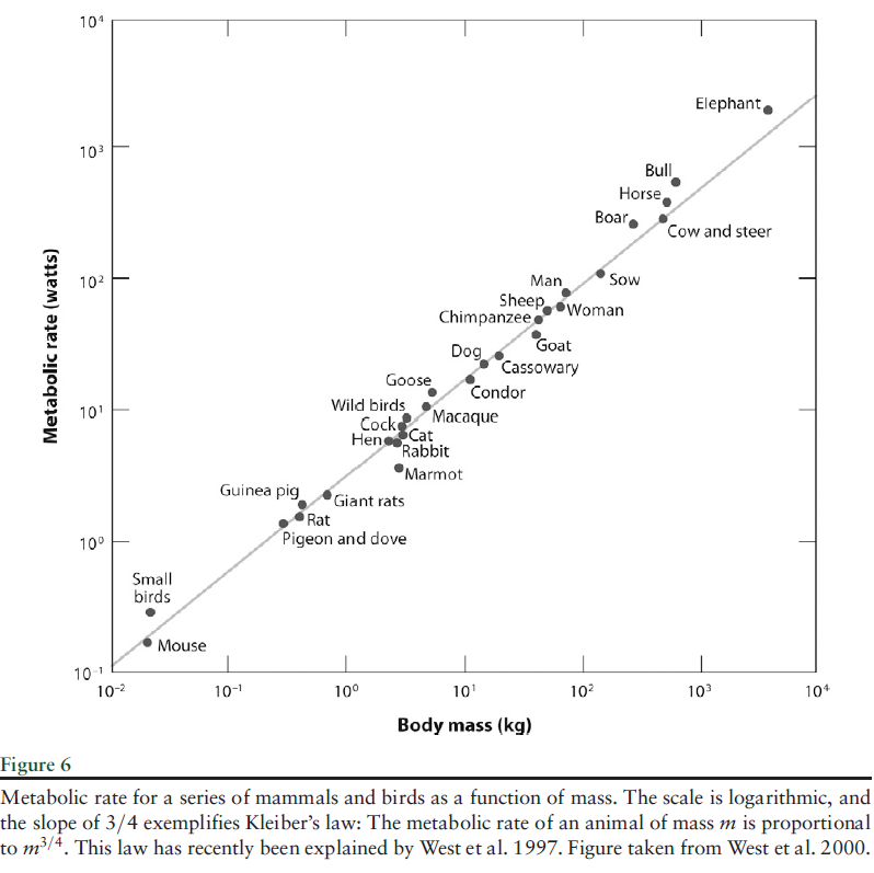
For example, the

..energy that an animal of mass M requires to live is proportional to M^3/4. This empirical regularity… has been explained only recently .. along the following lines: If one wants to design an optimal vascular system to send nutrients to the animal, one designs a fractal system, and maximum efficiency exactly delivers the M^3/4 law. In explaining the relationship between energy needs and mass, one should not become distracted by thinking about the specific features of animals, such as feathers and fur. Simple and deep principles underlie the regularities.

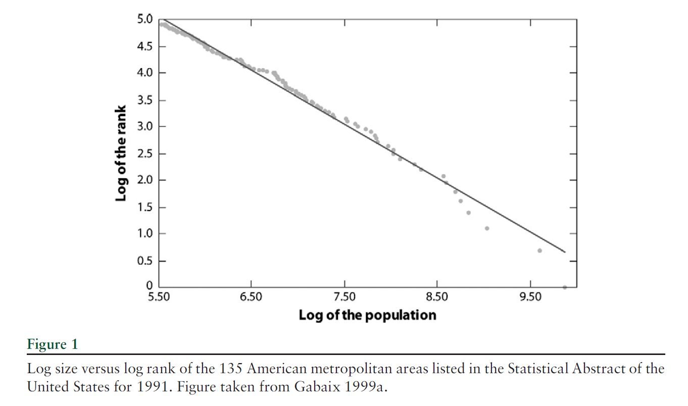
This type of relationship between variables also characterizes city population and rank, income and wealth distribution, visits to Internet blogs and blog rank, and many other phenomena.

Here is the graph of the power law for city size, developed much earlier by Gabaiux.

There are many valuable sections in Gabaix’s review article.

However, surely one of the most interesting is the inverse cubic law distribution of stock price fluctuations.

The tail distribution of short-term (15 s to a few days) returns has been analyzed in a series of studies on data sets, with a few thousands of data points (Jansen & de Vries 1991, Lux 1996, Mandelbrot 1963), then with an ever increasing number of data points: Mantegna& Stanley (1995) used 2 million data points, whereas Gopikrishnan et al. (1999) used over 200 million data points. Gopikrishnan et al. (1999) established a strong case for an inverse cubic PL of stock market returns. We let rt denote the logarithmic return over a time interval.. Gopikrishnan et al. (1999) found that the distribution function of returns for the 1000 largest U.S. stocks and several major international indices is

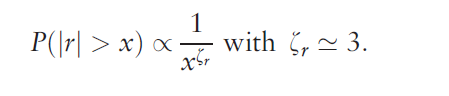
This relationship holds for positive and negative returns separately.

There is also an inverse half-cubic power law distribution of trading volume.

All this is fascinating, and goes beyond a sort of bestiary of weird social regularities. The holy grail here is, as Gabaix says, robust, detail-independent economic laws.

So with this goal in mind, we don’t object to the intricate details of the aggregation of power laws, or their potential genesis in proportional random growth. I was not aware, for example, that power laws are sustained through additive, multiplicative, min and max operations, possibly explaining why they are so widespread. Nor was I aware that randomly assigning multiplicative growth factors to a group of cities, individuals with wealth, and so forth can generate a power law, when certain noise elements are present.

And Gabaix is also aware that stock market crashes display many attributes that resolve or flow from power laws – so eventually it’s possible general mathematical principles could govern bubble dynamics, for example, somewhat independently of the specific context.

St. Petersburg Paradox

Power laws also crop up in places where standard statistical concepts fail. For example, while the expected or mean earnings from the St. Petersburg paradox coin flipping game does not exist, the probability distribution of payouts follow a power law.

Peter offers to let Paul toss a fair coin an indefinite number of times, paying him 2 coins if it comes up tails on the first toss, 4 coins if the first head comes up on the second toss, and 2ⁿ, if the first head comes up on the nth toss.

The paradox is that, with a fair coin, it is possible to earn an indefinitely large payout, depending on how long Paul is willing to flip coins. At the same time, behavioral experiments show that “Paul” is not willing to pay more than a token amount up front to play this game.

The probability distribution function of winnings is described by a power law, so that,

There is a high probability of winning a small amount of money. Sometimes, you get a few TAILS before that first HEAD and so you win much more money, because you win $2 raised to the number of TAILS plus one. Therefore, there is a medium probability of winning a large amount of money. Very infrequently you get a long sequence of TAILS and so you win a huge jackpot. Therefore, there is a very low probability of winning a huge amount of money. These frequent small values, moderately often medium values, and infrequent large values are analogous to the many tiny pieces, some medium sized pieces, and the few large pieces in a fractal object. There is no single average value that is the characteristic value of the winnings per game.

And, as Liebovitch and Scheurle illustrate with Monte Carlo simulations, as more games were played, the average winnings per game of the fractal St. Petersburg coin toss game …increase without bound.

So, neither the expected earnings nor the variance of average earnings exists as computable mathematical entities. And yet the PDF of the earnings is described by the formula Ax^-α  where α is near 1.

Closing Thoughts

One reason power laws are so pervasive in the real world is that, mathematically, they aggregate over addition and multiplication. So the sum of two variables described by a power law also is described by a power law, and so forth.

As far as their origin or principle of generation, it seems random proportional growth can explain some of the city size, wealth and income distribution power laws. But I hesitate to sketch the argument, because it seems somehow incomplete, requiring “frictions” or weird departures from a standard limit process.

In any case, I think those of us interested in forecasting should figure ways to integrate these unusual regularities into predictions.