Tag Archives: ARIMA modeling

Wrap on Exponential Smoothing

Here are some notes on essential features of exponential smoothing.

  1. Name. Exponential smoothing (ES) algorithms create exponentially weighted sums of past values to produce the next (and subsequent period) forecasts. So, in simple exponential smoothing, the recursion formula is Lt=αXt+(1-α)Lt-1 where α is the smoothing constant constrained to be within the interval [0,1], Xt is the value of the time series to be forecast in period t, and Lt is the (unobserved) level of the series at period t. Substituting the similar expression for Lt-1 we get Lt=αXt+(1-α) (αXt-1+(1-α)Lt-2)= αXt+α(1-α)Xt-1+(1-α)2Lt-2, and so forth back to L1. This means that more recent values of the time series X are weighted more heavily than values at more distant times in the past. Incidentally, the initial level L1 is not strongly determined, but is established by one ad hoc means or another – often by keying off of the initial values of the X series in some manner or another. In state space formulations, the initial values of the level, trend, and seasonal effects can be included in the list of parameters to be established by maximum likelihood estimation.
  2. Types of Exponential Smoothing Models. ES pivots on a decomposition of time series into level, trend, and seasonal effects. Altogether, there are fifteen ES methods. Each model incorporates a level with the differences coming as to whether the trend and seasonal components or effects exist and whether they are additive or multiplicative; also whether they are damped. In addition to simple exponential smoothing, Holt or two parameter exponential smoothing is another commonly applied model. There are two recursion equations, one for the level Lt and another for the trend Tt, as in the additive formulation, Lt=αXt+(1-α)(Lt-1+Tt-1) and Tt=β(Lt– Lt-1)+(1-β)Tt-1 Here, there are now two smoothing parameters, α and β, each constrained to be in the closed interval [0,1]. Winters or three parameter exponential smoothing, which incorporates seasonal effects, is another popular ES model.
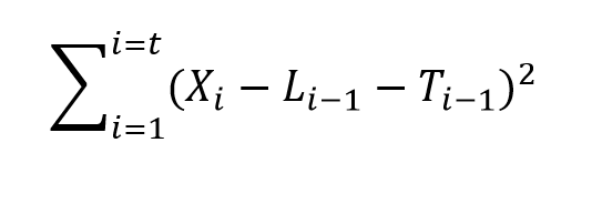
  3. Estimation of the Smoothing Parameters. The original method of estimating the smoothing parameters was to guess their values, following guidelines like “if the smoothing parameter is near 1, past values will be discounted further” and so forth. Thus, if the time series to be forecast was very erratic or variable, a value of the smoothing parameter which was closer to zero might be selected, to achieve a longer period average. The next step is to set up a sum of the squared differences of the within sample predictions and minimize these. Note that the predicted value of Xt+1 in the Holt or two parameter additive case is Lt+Tt, so this involves minimizing the expression Sqerroreq Currently, the most advanced method of estimating the value of the smoothing parameters is to express the model equations in state space form and utilize maximum likelihood estimation. It’s interesting, in this regard, that the error correction version of ES recursion equations are a bridge to this approach, since the error correction formulation is found at the very beginnings of the technique. Advantages of using the state space formulation and maximum likelihood estimation include (a) the ability to estimate confidence intervals for point forecasts, and (b) the capability of extending ES methods to nonlinear models.
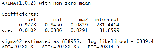
  4. Comparison with Box-Jenkins or ARIMA models. ES began as a purely applied method developed for the US Navy, and for a long time was considered an ad hoc procedure. It produced forecasts, but no confidence intervals. In fact, statistical considerations did not enter into the estimation of the smoothing parameters at all, it seemed. That perspective has now changed, and the question is not whether ES has statistical foundations – state space models seem to have solved that. Instead, the tricky issue is to delineate the overlap and differences between ES and ARIMA models. For example, Gardner makes the statement that all linear exponential smoothing methods have equivalent ARIMA models. Hyndman points out that the state space formulation of ES models opens the way for expressing nonlinear time series – a step that goes beyond what is possible in ARIMA modeling.
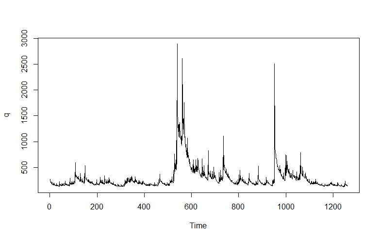
  5. The Importance of Random Walks. The random walk is a forecasting benchmark. In an early paper, Muth showed that a simple exponential smoothing model provided optimal forecasts for a random walk. The optimal forecast for a simple random walk is the current period value. Things get more complicated when there is an error associated with the latent variable (the level). In that case, the smoothing parameter determines how much of the recent past is allowed to affect the forecast for the next period value.
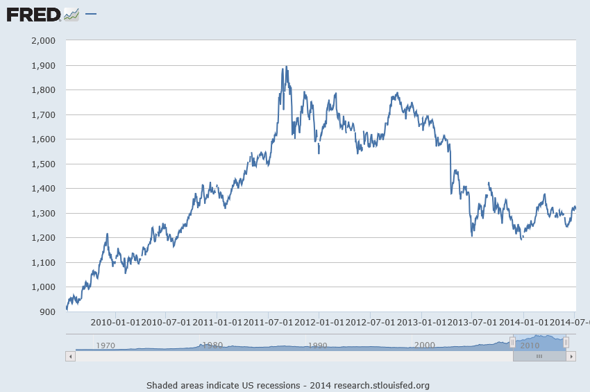
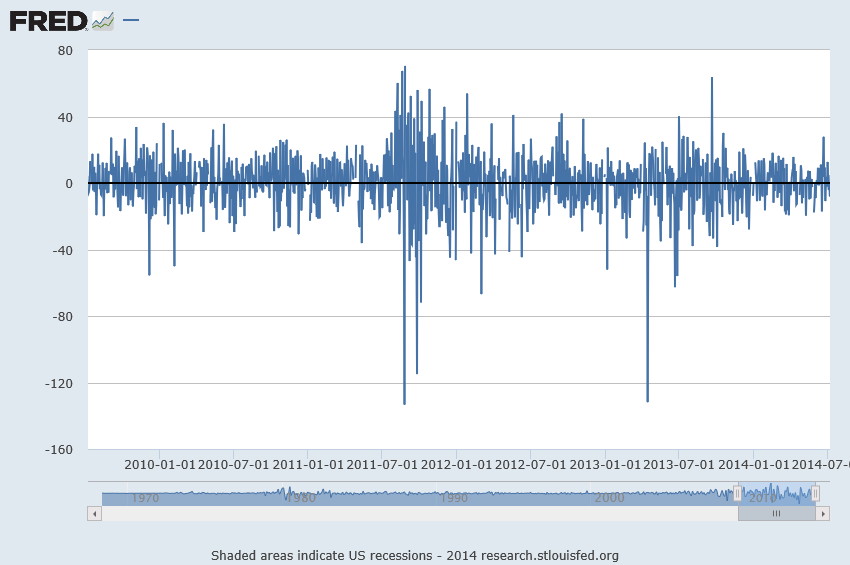
  6. Random Walks With Drift. A random walk with drift, for which a two parameter ES model can be optimal, is an important form insofar as many business and economic time series appear to be random walks with drift. Thus, first differencing removes the trend, leaving ideally white noise. A huge amount of ink has been spilled in econometric investigations of “unit roots” – essentially exploring whether random walks and random walks with drift are pretty much the whole story when it comes to major economic and business time series.
  7. Advantages of ES. ES is relatively robust, compared with ARIMA models, which are sensitive to mis-specification. Another advantage of ES is that ES forecasts can be up and running with only a few historic observations. This comment applied to estimation of the level and possibly trend, but does not apply in the same degree to the seasonal effects, which usually require more data to establish. There are a number of references which establish the competitive advantage in terms of the accuracy of ES forecasts in a variety of contexts.
  8. Advanced Applications.The most advanced application of ES I have seen is the research paper by Hyndman et al relating to bagging exponential smoothing forecasts.

The bottom line is that anybody interested in and representing competency in business forecasting should spend some time studying the various types of exponential smoothing and the various means to arrive at estimates of their parameters.

For some reason, exponential smoothing reaches deep into actual process in data generation and consistently produces valuable insights into outcomes.

More Blackbox Analysis – ARIMA Modeling in R

Automatic forecasting programs are seductive. They streamline analysis, especially with ARIMA (autoregressive integrated moving average) models. You have to know some basics – such as what the notation ARIMA(2,1,1) or ARIMA(p,d,q) means. But you can more or less sidestep the elaborate algebra – the higher reaches of equations written in backward shift operators – in favor of looking at results. Does the automatic ARIMA model selection predict out-of-sample, for example?

I have been exploring the Hyndman R Forecast package – and other contributors, such as George Athanasopoulos, Slava Razbash, Drew Schmidt, Zhenyu Zhou, Yousaf Khan, Christoph Bergmeir, and Earo Wang, should be mentioned.

A 76 page document lists the routines in Forecast, which you can download as a PDF file.

This post is about the routine auto.arima(.) in the Forecast package. This makes volatility modeling – a place where Box Jenkins or ARIMA modeling is relatively unchallenged – easier. The auto.arima(.) routine also encourages experimentation, and highlights the sharp limitations of volatility modeling in a way that, to my way of thinking, is not at all apparent from the extensive and highly mathematical literature on this topic.

Daily Gold Prices

I grabbed some data from FRED – the Gold Fixing Price set at 10:30 A.M (London time) in London Bullion Market, based in U.S. Dollars.

GOLDAMGBD228NLBM

Now the price series shown in the graph above is a random walk, according to auto.arima(.).

In other words, the routine indicates that the optimal model is ARIMA(0,1,0), which is to say that after differencing the price series once, the program suggests the series reduces to a series of independent random values. The automatic exponential smoothing routine in Forecast is ets(.). Running this confirms that simple exponential smoothing, with a smoothing parameter close to 1, is the optimal model – again, consistent with a random walk.

Here’s a graph of these first differences.

1stdiffgold

But wait, there is a clustering of volatility of these first differences, which can be accentuated if we square these values, producing the following graph.

volatilityGP

Now in a more or less textbook example, auto.arima(.) develops the following ARIMA model for this series

model

Thus, this estimate of the volatility of the first differences of gold price is modeled as a first order autoregressive process with two moving average terms.

Here is the plot of the fitted values.

Rplot1

Nice.

But of course, we are interested in forecasting, and the results here are somewhat more disappointing.

Basically, this type of model makes a horizontal line prediction at a certain level, which is higher when the past values have been higher.

This is what people in quantitative finance call “persistence” but of course sometimes new things happen, and then these types of models do not do well.

From my research on the volatility literature, it seems that short period forecasts are better than longer period forecasts. Ideally, you update your volatility model daily or at even higher frequencies, and it’s likely your one or two period ahead (minutes, hours, a day) will be more accurate.

Incidentally, exponential smoothing in this context appears to be a total fail, again suggesting this series is a simple random walk.

Recapitulation

There is more here than meets the eye.

First, the auto.arima(.) routines in the Hyndman R Forecast package do a competent job of modeling the clustering of higher first differences of the gold price series here. But, at the same time, they highlight a methodological point. The gold price series really has nonlinear aspects that are not adequately commanded by a purely linear model. So, as in many approximations, the assumption of linearity gets us some part of the way, but deeper analysis indicates the existence of nonlinearities. Kind of interesting.

Of course, I have not told you about the notation ARIMA(p,d,q). Well, p stands for the order of the autoregressive terms in the equation, q stands for the moving average terms, and d indicates the times the series is differenced to reduce it to a stationary time series. Take a look at Forecasting: principles and practice – the free forecasting text of Hyndman and Athanasopoulos – in the chapter on ARIMA modeling for more details.

Incidentally, I think it is great that Hyndman and some of his collaborators are providing an open source, indeed free, forecasting package with automatic forecasting capabilities, along with a high quality and, again, free textbook on forecasting to back it up. Eventually, some of these techniques might get dispersed into the general social environment, potentially raising the level of some discussions and thinking about our common future.

And I guess also I have to say that, ultimately, you need to learn the underlying theory and struggle with the algebra some. It can improve one’s ability to model these series.

More on Automatic Forecasting Packages – Autobox Gold Price Forecasts

Yesterday, my post discussed the statistical programming language R and Rob Hyndman’s automatic forecasting package, written in R – facts about this program, how to download it, and an application to gold prices.

In passing, I said I liked Hyndman’s disclosure of his methods in his R package and “contrasted” that with leading competitors in the automatic forecasting market space –notably Forecast Pro and Autobox.

This roused Tom Reilly, currently Senior Vice-President and CEO of Automatic Forecast Systems – the company behind Autobox.

62_tom

Reilly, shown above, wrote  –

You say that Autobox doesn’t disclose its methods.  I think that this statement is unfair to Autobox.  SAS tried this (Mike Gilliland) on the cover of his book showing something purporting to a black box.  We are a white box.  I just downloaded the GOLD prices and recreated the problem and ran it. If you open details.htm it walks you through all the steps of the modeling process.  Take a look and let me know your thoughts.  Much appreciated!

AutoBox Gold Price Forecast

First, disregarding the issue of transparency for a moment, let’s look at a comparison of forecasts for this monthly gold price series (London PM fix).

A picture tells the story (click to enlarge).

ABFPHcomp

So, for this data, 2007 to early 2011, Autobox dominates. That is, all forecasts are less than the respective actual monthly average gold prices. Thus, being linear, if one forecast method is more inaccurate than another for one month, that method is less accurate than the forecasts generated by this other approach for the entire forecast horizon.

I guess this does not surprise me. Autobox has been a serious contender in the M-competitions, for example, usually running just behind or perhaps just ahead of Forecast Pro, depending on the accuracy metric and forecast horizon. (For a history of these “accuracy contests” see Markridakis and Hibon’s article on M3).

And, of course, this is just one of many possible forecasts that can be developed with this time series, taking off from various ending points in the historic record.

The Issue of Transparency

In connection with all this, I also talked with Dave Reilly, a founding principal of Autobox, shown below.

DaveReilly

Among other things, we went over the “printout” Tom Reilly sent, which details the steps in the estimation of a final time series model to predict these gold prices.

A blog post on the Autobox site is especially pertinent, called Build or Make your own ARIMA forecasting model? This discussion contains two flow charts which describe the process of building a time series model, I reproduce here, by kind permission.

The first provides a plain vanilla description of Box-Jenkins modeling.

Rflowchart1

The second flowchart adds steps revised for additions by Tsay, Tiao, Bell, Reilly & Gregory Chow (ie chow test).

Rflowchart2

Both start with plotting the time series to be analyzed and calculating the autocorrelation and partial autocorrelation functions.

But then additional boxes are added for accounting for and removing “deterministic” elements in the time series and checking for the constancy of parameters over the sample.

The analysis run Tom Reilly sent suggests to me that “deterministic” elements can mean outliers.

Dave Reilly made an interesting point about outliers. He suggested that the true autocorrelation structure can be masked or dampened in the presence of outliers. So the tactic of specifying an intervention variable in the various trial models can facilitate identification of autoregressive lags which otherwise might appear to be statistically not significant.

Really, the point of Autobox model development is to “create an error process free of structure.” That a Dave Reilly quote.

So, bottom line, Autobox’s general methods are well-documented. There is no problem of transparency with respect to the steps in the recommended analysis in the program. True, behind the scenes, comparisons are being made and alternatives are being rejected which do not make it to the printout of results. But you can argue that any commercial software has to keep some kernel of its processes proprietary.

I expect to be writing more about Autobox. It has a good track record in various forecasting competitions and currently has a management team that actively solicits forecasting challenges.