Tag Archives: Data Science

Ebola and Data Analysis

Data analysis and predictive analytics can support national and international responses to ebola.

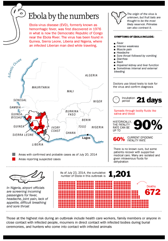
One of the primary ways at present is by verifying and extrapolating the currently exponential growth of ebola in affected areas – especially in Monrovia, the capital of Liberia, as well as Sierra Leone, Guinea, Nigeria, and the Democratic Republic of the Congo.

At this point, given data from the World Health Organization (WHO) and other agencies, predictive modeling can be as simple as in the following two charts, developed from the data compiled (and documented) in the Wikipedia site.

The first charts datapoints from the end of the months of May through August of this year.

Ebolacasesmodeling

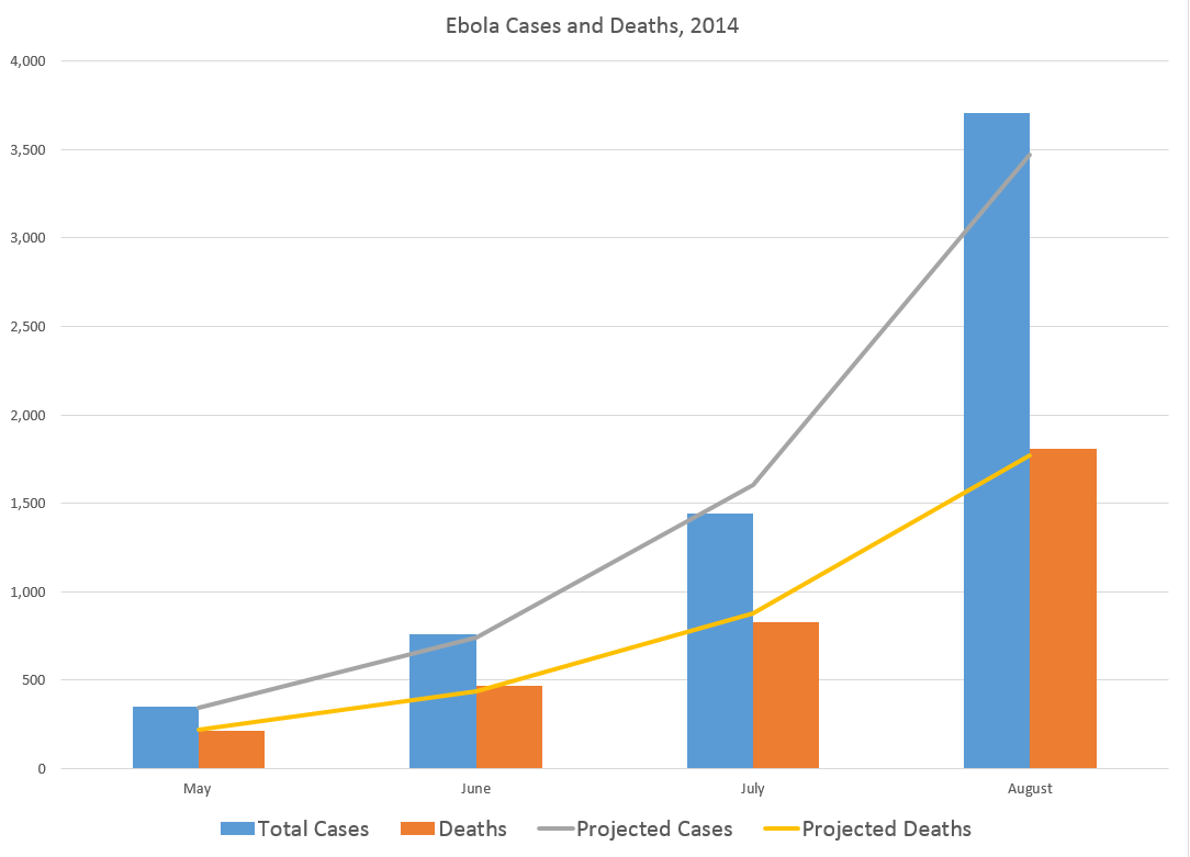
The second chart extrapolates an exponential fit to these cases, shown in the lines in the above figure, by month through December 2014.

Ebolaprojections

So by the end of this year, if this epidemic courses unchecked, without the major public health investments necessary in terms of hospital beds, supplies, medical and supporting personnel, including military or police forces to maintain public order in some of the worst-hit areas – there will be nearly 80,000 cases and approximately 30,000 deaths, by this simple extrapolation.

A slightly more sophisticated analysis by Geert Barentsen, utilizing data within calendar months as well, concludes that currently Ebola cases have a doubling time of 29 days.

One possibly positive aspect of these projections is the death rate declines from around 60 to 40 percent, from May through December 2014.

However, if the epidemic continues through 2015 at this rate, the projections suggest there will be more than 300 million cases.

World Health Organization (WHO) estimates released the first week of September indicate nearly 2,400 deaths. Total numbers of cases from the same period in early September is 4,846. So the projections are on track so far.

And, if you wish, you can validate these crude data analytics with reference to modeling using the classic compartment approach and other more advanced setups. See, for example, Disease modelers project a rapidly rising toll from Ebola or the recent New York Times article.

Visual Analytics

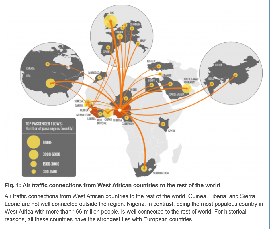
There have been advanced modeling efforts at discovering the possibilities of transmission of Ebola through persons traveling by air to other affected areas.

Here is a chart from Assessing the International Spreading Risk Associated with the 2014 West African Ebola Outbreak.

ebolaairroutes

As a data and forecasting analyst, I am not specially equipped to comment on the conditions which make transmission of this disease particularly dangerous. But I think, to some extent, it’s not rocket science.

Crowded conditions in many African cities, low educational attainment, poverty, poor medical infrastructure, rapid population growth – all these factors contribute to the high basic reproductive number of the disease in this outbreak. And, if the numbers of cases increase toward 100,000, the probability that some of the affected individuals will travel elsewhere grows, particularly when efforts to quarantine areas seem heavy-handed and, given little understanding of modern disease models in the affected populations, possibly suspicious.

There is a growing response from agencies and places as widely ranging as the Gates Foundation and Cuba, but what I read is that a military-type operation will be necessary to bring the epidemic under control. I suppose this means command-and-control centers must be established, set procedures must be implemented when cases are identified, adequate field hospitals need to be established, enough medical personnel must be deployed, and so forth. And if there are potential vaccines, these probably will be expensive to administer in early stages.

These thoughts are suggested by the numbers. So far, the numbers speak for themselves.

E-Commerce Apps for Website Optimization

There are dozens of web-based metrics for assessing ecommerce sites, but in the final analysis it probably just comes down to “conversion” rate. How many visitors to your ecommerce site end up buying your product or service?

Many factors come into play – such as pricing structure, product quality, customer service, and reputation.

But real-time predictive analytics plays an increasing role, according to How Predictive Analytics Is Transforming eCommerce & Conversion Rate Optimization. The author – Peep Laja – seems fond of Lattice, writing that,

Lattice has researched how leading companies like Amazon & Netflix are using predictive analytics to better understand customer behavior, in order to develop a solution that helps sales professionals better qualify their leads.

AZNF

Laja also notes impressive success stories, such as Macy’s – which clocked an 8 to 12 percent increase in online sales by combining browsing behavior within product categories and sending targeted emails by customer segment.

Google and Bandit Testing

I find the techniques associated with A/B or Bandit testing fascinating.

Google is at the forefront of this – the experimental testing of webpage design and construction.

Let me recommend readers directly to Google Analytics – the discussion headed by Overview of Content Experiments.

What is Bandit Testing?

Well, the Google presentation Multi-armed Bandits is really clear.

This is a fun topic.

So suppose you have a row of slot machine (“one-armed bandits”) and you know each machine has different probabilities and size of payouts. How do you decide which machine to favor, after a period of experimentation?

This is the multi-armed bandit or simply bandit problem, and is mathematically very difficult.

[The bandit problem] was formulated during the [second world] war, and efforts to solve it so sapped the energies and minds of Allied analysts that the suggestion was made that the problem be dropped over Germany, as the ultimate instrument of intellectual sabotage.

The Google discussion illustrates a Bayesian algorithm with simulations, showing that updating the probabilities and flow of traffic to what appear to be the most attractive web pages results, typically, in more rapid solutions that classical statistical experiments (generally known as A/B testing after “showroom A” and “showroom B”).

Suppose you’ve got a conversion rate of 4% on your site. You experiment with a new version of the site that actually generates conversions 5% of the time. You don’t know the true conversion rates of course, which is why you’re experimenting, but let’s suppose you’d like your experiment to be able to detect a 5% conversion rate as statistically significant with 95% probability. A standard power calculation1 tells you that you need 22,330 observations (11,165 in each arm) to have a 95% chance of detecting a .04 to .05 shift in conversion rates. Suppose you get 100 sessions per day to the experiment, so the experiment will take 223 days to complete. In a standard experiment you wait 223 days, run the hypothesis test, and get your answer.

Now let’s manage the 100 sessions each day through the multi-armed bandit. On the first day about 50 sessions are assigned to each arm, and we look at the results. We use Bayes’ theorem to compute the probability that the variation is better than the original2. One minus this number is the probability that the original is better. Let’s suppose the original got really lucky on the first day, and it appears to have a 70% chance of being superior. Then we assign it 70% of the traffic on the second day, and the variation gets 30%. At the end of the second day we accumulate all the traffic we’ve seen so far (over both days), and recompute the probability that each arm is best. That gives us the serving weights for day 3. We repeat this process until a set of stopping rules has been satisfied (we’ll say more about stopping rules below).

Figure 1 shows a simulation of what can happen with this setup. In it, you can see the serving weights for the original (the black line) and the variation (the red dotted line), essentially alternating back and forth until the variation eventually crosses the line of 95% confidence. (The two percentages must add to 100%, so when one goes up the other goes down). The experiment finished in 66 days, so it saved you 157 days of testing.

This Figure 1 chart is as follows.

2armThis is obviously just one outcome, but running this test many times verifies that in a majority of cases, the Google algorithm results in substantial shortening of test time, compared with an A/B test. In addition, if actual purchases are the meaning of “conversion” here, revenues are higher.

This naturally generalizes to any number of “arms” or slot machines.

Apparently, investors have put nearly $200 million in 2014 into companies developing predictive apps for ecommerce.

And, on the other side of the ledger, there are those who say that the mathematical training of people who might use these apps is still sub-par, and that the full potential of these techniques may not be realized in many cases.

The deeper analytics of the Google application is fascinating. It involves Monte Carlo simulation to integrate products of conditional and prior distributions, after new data comes in.

My math intuition, such as it is, suggests that this approach has wider applications. Why could it not, for example, be utilized for new products, where there might be two states, i.e. the product is a winner (following similar products in ramping up) or a loser? It’s also been used in speeding up health trials – an application of Bayesian techniques.

Top graphic from the One Hour Professor

e-commerce and Forecasting

The Census Bureau announced numbers from its latest e-commerce survey August 15.

The basic pattern continues. US retail e-commerce sales increased about 16 percent on a year-over-year basis from the second quarter of 2013. By comparison, total retail sales for the second quarter 2014 increased just short of 5 percent on a year-over-year basis.

 ecommercepercent

As with other government statistics relating to IT (information technology), one can quarrel with the numbers (they may, for example, be low), but there is impressive growth no matter how you cut it.

Some of the top e-retailers from the standpoint of clicks and sales numbers are listed in Panagiotelis et al. Note these are sample data, from comScore with the totals for each company or site representing a small fraction of their actual 2007 online sales.

eretailers

Forecasting Issues

Forecasting issues related to e-commerce run the gamut.

Website optimization and target marketing raise questions such as the profitability of “stickiness” to e-commerce retailers. There are advanced methods to tease out nonlinear, nonnormal multivariate relationships between, say, duration and page views and the decision to purchase – such as copulas previously applied in financial risk assessment and health studies.

Mobile e-commerce is a rapidly growing area with special platform and communications characteristics all its own.

Then, there are the pros and cons of expanding tax collection for online sales.

All in all, Darrell Rigby’s article in the Harvard Business Review – The Future of Shopping – is hard to beat. Traditional retailers generally have to move to a multi-channel model, supplementing brick-and-mortar stores with online services.

I plan several posts on these questions and issues, and am open for your questions.

Top graphic by DIGISECRETS

First peek at “Revolutions” exhibit at Computer History Museum with Woz

I think Steve Wozniack is a kind of hero – from what I understand still connected with helping young people and in this video, giving some “straight from the horses mouth” commentary on the history of computing. 

And I am making plans to return to pattern on this blog.

That is, I will be focusing on issues tagged a couple of posts ago – namely geopolitical risks (ebola, unfolding warfare at several locations), the emerging financial bubble, and 21st century data analysis and forecasting techniques.

But, I think perhaps a little like Woz, I am a technological utopian at heart. If we could develop technologies which would allow younger people around the globe some type of “hands on” potential – maybe a little like the old computer systems which these technical leaders, now mostly all billionaires, had access to – if we could find these new technologies, I think we could knit the world together once again. Of course, this idea devolves when the “hands on” potential is occasioned by weapons – and the image of the child soldiers in Africa comes to mind.

I like the part in the video where Woz describes using a nonstandard card punch machine to get his card deck in order at Berkeley – the part where he draws a lesson about learning to do what works, not what the symbols indicate.

Links early August 2014

Economy/Business

Economists React to July’s Jobs Report: ‘Not Weak, But…’

U.S. nonfarm employers added 209,000 jobs in July, slightly below forecasts and slower than earlier gains, while the unemployment rate ticked up to 6.2% from June. But employers have now added 200,000 or more jobs in six consecutive months for the first time since 1997.

The most important charts to see before the huge July jobs report – interesting to see what analysts were looking at just before the jobs announcement.

Despite sharp selloff, too early to worry about a correction

Venture Capital: Deals Beyond the Valley

7 Most Expensive Luxury Cars

BMW

Base price $136,000.

Contango And Backwardation Strategy For VIX ETFs Here you go!

Climate/Weather

Horrid California Drought Gets Worse Has a map showing drought conditions at intervals since 2011, dramatic.

IT

Amazon’s Cloud Is Growing So Fast It’s Scaring Shareholders

Amazon has pulled off a pretty amazing trick over the past decade. It’s invented and then built a nearly $5 billion cloud computing business catering to fickle software developers and put the rest of the technology industry on the defensive. Big enterprise software companies such as IBM and HP and even Google are playing catchup, even as they acknowledge that cloud computing is the tech industry’s future.

But what kind of a future is that to be? Yesterday Amazon said that while its cloud business grew by 90 percent last year, it was significantly less profitable. Amazon’s AWS cloud business makes up the majority of a balance sheet item it labels as “other” (along with its credit card and advertising revenue) and that revenue from that line of business grew by 38 percent. Last quarter, revenue grew by 60 percent. In other words, Amazon is piling on customers faster than it’s adding dollars to its bottom line.

The Current Threat

Infographic: Ebola By the Numbers

ebola

Data Science

Statistical inference in massive data sets Interesting and applicable procedure illustrated with Internet traffic numbers.

Semiconductor Cycles

I’ve been exploring cycles in the semiconductor, computer and IT industries generally for quite some time.

Here is an exhibit I prepared in 2000 for a magazine serving the printed circuit board industry.

semicycle

The data come from two sources – the Semiconductor Industry Association (SIA) World Semiconductor Trade Statistics database and the Census Bureau manufacturing series for computer equipment.

This sort of analytics spawned a spate of academic research, beginning more or less with the work of Tan and Mathews in Australia.

One of my favorites is a working paper released by DRUID – the Danish Research Unit for Industrial Dynamics called Cyclical Dynamics in Three Industries. Tan and Mathews consider cycles in semiconductors, computers, and what they call the flat panel display industry. They start with quoting “industry experts” and, specifically, some of my work with Economic Data Resources on the computer (PC) cycle. These researchers went on to publish in the Journal of Business Research and Technological Forecasting and Social Change in 2010. A year later in 2011, Tan published an interesting article on the sequencing of cyclical dynamics in semiconductors.

Essentially, the appearance of cycles and what I have called quasi-cycles or pseudo-cycles in the semiconductor industry and other IT categories, like computers, result from the interplay of innovation, investment, and pricing. In semiconductors, for example, Moore’s law – which everyone always predicts will fail at some imminent future point – indicates that continuing miniaturization will lead to periodic reductions in the cost of information processing. At some point in the 1980’s, this cadence was firmly established by introductions of new microprocessors by Intel roughly every 18 months. The enhanced speed and capacity of these microprocessors – the “central nervous system” of the computer – was complemented by continuing software upgrades, and, of course, by the movement to graphical interfaces with Windows and the succession of Windows releases.

Back along the supply chain, semiconductor fabs were retooling periodically to produce chips with more and more transitors per volume of silicon. These fabs were, simply put, fabulously expensive and the investment dynamics factors into pricing in semiconductors. There were famous gluts, for example, of memory chips in 1996, and overall the whole IT industry led the recession of 2001 with massive inventory overhang, resulting from double booking and the infamous Y2K scare.

Statistical Modeling of IT Cycles

A number of papers, summarized in Aubrey deploy VAR (vector autoregression) models to capture leading indicators of global semiconductor sales. A variant of these is the Bayesian VAR or BVAR model. Basically, VAR models sort of blindly specify all possible lags for all possible variables in a system of autoregressive models. Of course, some cutoff point has to be established, and the variables to be included in the VAR system have to be selected by one means or another. A BVAR simply reduces the number of possibilities by imposing, for example, sign constraints on the resulting coefficients, or, more ambitiously, employs some type of prior distribution for key variables.

Typical variables included in these models include:

  • WSTS monthly semiconductor shipments (now by subscription only from SIA)
  • Philadelphia semiconductor index (SOX) data
  • US data on various IT shipments, orders, inventories from M3
  • data from SEMI, the association of semiconductor equipment manufacturers

Another tactic is to filter out low and high frequency variability in a semiconductor sales series with something like the Hodrick-Prescott (HP) filter, and then conduct a spectral analysis.

Does the Semiconductor/Computer/IT Cycle Still Exist?

I wonder whether academic research into IT cycles is a case of “redoubling one’s efforts when you lose sight of the goal,” or more specifically, whether new configurations of forces are blurring the formerly fairly cleanly delineated pulses in sales growth for semiconductors, computers, and other IT hardware.

“Hardware” is probably a key here, since there have been big changes since the 1990’s and early years of this brave new century.

For one thing, complementarities between software and hardware upgrades seem to be breaking down. This began in earnest with the development of virtual servers – software which enabled many virtual machines on the same hardware frame, in part because the underlying circuitry was so massively powerful and high capacity now. Significant declines in the growth of sales of these machines followed on wide deployment of this software designed to achieve higher efficiencies of utilization of individual machines.

Another development is cloud computing. Running the data side of things is gradually being taken away from in-house IT departments in companies and moved over to cloud computing services. Of course, critical data for a company is always likely to be maintained in-house, but the need for expanding the number of big desktops with the number of employees is going away – or has indeed gone away.

At the same time, tablets, Apple products and Android machines, created a wave of destructive creation in people’s access to the Internet, and, more and more, for everyday functions like keeping calendars, taking notes, even writing and processing photos.

But note – I am not studding this discussion with numbers as of yet.

I suspect that underneath all this change it should be possible to identify some IT invariants, perhaps in usage categories, which continue to reflect a kind of pulse and cycle of activity.

Some Cycle Basics

A Fourier analysis is one of the first steps in analyzing cycles.

Take sunspots, for example,

There are extensive historic records on the annual number of sunspots, dating back to 1700. The annual data shown in the following graph dates back to 1700, and is currently maintained by the Royal Belgium Observatory.

sunspots

This series is relatively stationary, although there may be a slight trend if you cut this span of data off a few years before the present.

In any case, the kind of thing you get with a Fourier analysis looks like this.

spectralsunspots

This shows the power or importance of the cycles/year numbers, and maxes out at around 0.09.

These data can be recalibrated into the following chart, which highlights the approximately 11 year major cycle in the sunspot numbers.

sunspotsperiodogramyr

Now it’s possible to build a simple regression model with a lagged explanatory variable to make credible predictions. A lag of eleven years produces the following in-sample and out-of-sample fits. The regression is estimated over data to 1990, and, thus, the years 1991 through 2013 are out-of-sample.

LaggedModel

It’s obvious this sort of forecasting approach is not quite ready for prime-time television, even though it performs OK on several of the out-of-sample years after 1990.

But this exercise does highlight a couple of things.

First, the annual number of sunspots is broadly cyclical in this sense. If you try the same trick with lagged values for the US “business cycle” the results will be radically worse. At least with the sunspot data, most of the fluctuations have timing that is correctly predicted, both in-sample (1990 and before) and out-of-sample (1991-2013).

Secondly, there are stochastic elements to this solar activity cycle. The variation in amplitude is dramatic, and, indeed, the latest numbers coming in on sunspot activity are moving to much lower levels, even though the cycle is supposedly at its peak.

I’ve reviewed several papers on predicting the sunspot cycle. There are models which are more profoundly inspired by the possible physics involved – dynamo dynamics for example. But for my money there are basic models which, on a one-year-ahead basis, do a credible job. More on this forthcoming.

Video Friday – Andrew Ng’s Machine Learning Course

Well, I signed up for Andrew Ng’s Machine Learning Course at Stanford. It began a few weeks ago, and is a next generation to lectures by Ng circulating on YouTube. I’m going to basically audit the course, since I started a little late, but I plan to take several of the exams and work up a few of the projects. This course provides a broad introduction to machine learning, datamining, and statistical pattern recognition. Topics include: (i) Supervised learning (parametric/non-parametric algorithms, support vector machines, kernels, neural networks). (ii) Unsupervised learning (clustering, dimensionality reduction, recommender systems, deep learning). (iii) Best practices in machine learning (bias/variance theory; innovation process in machine learning and AI). The course will also draw from numerous case studies and applications, so that you’ll also learn how to apply learning algorithms to building smart robots (perception, control), text understanding (web search, anti-spam), computer vision, medical informatics, audio, database mining, and other areas. I like the change in format. The YouTube videos circulating on the web are lengthly, and involve Ng doing derivations on white boards. This is a more informal, expository format. Here is a link to a great short introduction to neural networks. Ngrobot Click on the link above this picture, since the picture itself does not trigger a YouTube. Ng’s introduction on this topic is fairly short, so here is the follow-on lecture, which starts the task of representing or modeling neural networks. I really like the way Ng approaches this is grounded in biology. I believe there is still time to sign up. Comment on Neural Networks and Machine Learning I can’t do much better than point to Professor Ng’s definition of machine learning – Machine learning is the science of getting computers to act without being explicitly programmed. In the past decade, machine learning has given us self-driving cars, practical speech recognition, effective web search, and a vastly improved understanding of the human genome. Machine learning is so pervasive today that you probably use it dozens of times a day without knowing it. Many researchers also think it is the best way to make progress towards human-level AI. In this class, you will learn about the most effective machine learning techniques, and gain practice implementing them and getting them to work for yourself. More importantly, you’ll learn about not only the theoretical underpinnings of learning, but also gain the practical know-how needed to quickly and powerfully apply these techniques to new problems. Finally, you’ll learn about some of Silicon Valley’s best practices in innovation as it pertains to machine learning and AI. And now maybe this is the future – the robot rock band.

Video Friday – Quantum Computing

I’m instituting Video Friday. It’s the end of the work week, and videos introduce novelty and pleasant change in communications.

And we can keep focusing on matters related to forecasting applications and data analytics, or more generally on algorithmic guides to action.

Today I’m focusing on D-Wave and quantum computing. This could well could take up several Friday’s, with cool videos on underlying principles and panel discussions with analysts from D-Wave, Google and NASA. We’ll see. Probably, I will treat it as a theme, returning to it from time to time.

A couple of introductory comments.

First of all, David Wineland won a Nobel Prize in physics in 2012 for his work with quantum computing. I’ve heard him speak, and know members of his family. Wineland did his work at the NIST Laboratories in Boulder, the location for Eric Cornell’s work which was awarded a Nobel Prize in 2001.

I mention this because understanding quantum computing is more or less like trying to understand quantum physics, and, there, I think engineering has a role to play.

The basic concept is to exploit quantum superimposition, or perhaps quantum entanglement, as a kind of parallel processor. The qubit, or quantum bit, is unlike the bit of classical computing. A qubit can be both 0 and 1 simultaneously, until it’s quantum wave equation is collapsed or dispersed by measurement. Accordingly, the argument goes, qubits scale as powers of 2, and a mere 500 qubits could more than encode all atoms in the universe. Thus, quantum computers may really shine at problems where you have to search through all different combinations of things.

But while I can write the quantum wave equation of Schrodinger, I don’t really understand it in any basic sense. It refers to a probability wave, whatever that is.

Feynman, whose lectures (and tapes or CD’s) on physics I proudly own, says it is pointless to try to “understand” quantum weirdness. You have to be content with being able to predict outcomes of quantum experiments with the apparatus of the theory. The theory is highly predictive and quite successful, in that regard.

So I think D-Wave is really onto something. They are approaching the problem of developing a quantum computer technologically.

Here is a piece of fluff Google and others put together about their purchase of a D-Wave computer and what’s involved with quantum computing.

OK, so now here is Eric Ladizinsky in a talk from April of this year on Evolving Scalable Quantum Computers. I can see why Eric gets support from DARPA and Bezos, a range indeed. You really get the “ah ha” effect listening to him. For example, I have never before heard a coherent explanation of how the quantum weirdness typical for small particles gets dispersed with macroscopic scale objects, like us. But this explanation, which is mathematically based on the wave equation, is essential to the D-Wave technology.

It takes more than an hour to listen to this video, but, maybe bookmark it if you pass on from a full viewing, since I assure you that this is probably the most substantive discussion I have yet found on this topic.

But is D-Wave’s machine a quantum computer?

Well, they keep raising money.

D-Wave Systems raises $30M to keep commercializing its quantum computer

But this infuriates some in the academic community, I suspect, who distrust the announcement of scientific discovery by the Press Release.

There is a brilliant article recently in Wired on D-Wave, which touches on a recent challenge to its computational prowess (See Is D-Wave’s quantum computer actually a quantum computer?)

The Wired article gives Geordie Rose, a D-Wave founder, space to rebut at which point these excellent comments can be found:

Rose’s response to the new tests: “It’s total bullshit.”

D-Wave, he says, is a scrappy startup pushing a radical new computer, crafted from nothing by a handful of folks in Canada. From this point of view, Troyer had the edge. Sure, he was using standard Intel machines and classical software, but those benefited from decades’ and trillions of dollars’ worth of investment. The D-Wave acquitted itself admirably just by keeping pace. Troyer “had the best algorithm ever developed by a team of the top scientists in the world, finely tuned to compete on what this processor does, running on the fastest processors that humans have ever been able to build,” Rose says. And the D-Wave “is now competitive with those things, which is a remarkable step.”

But what about the speed issues? “Calibration errors,” he says. Programming a problem into the D-Wave is a manual process, tuning each qubit to the right level on the problem-solving landscape. If you don’t set those dials precisely right, “you might be specifying the wrong problem on the chip,” Rose says. As for noise, he admits it’s still an issue, but the next chip—the 1,000-qubit version codenamed Washington, coming out this fall—will reduce noise yet more. His team plans to replace the niobium loops with aluminum to reduce oxide buildup….

Or here’s another way to look at it…. Maybe the real problem with people trying to assess D-Wave is that they’re asking the wrong questions. Maybe his machine needs harder problems.

On its face, this sounds crazy. If plain old Intels are beating the D-Wave, why would the D-Wave win if the problems got tougher? Because the tests Troyer threw at the machine were random. On a tiny subset of those problems, the D-Wave system did better. Rose thinks the key will be zooming in on those success stories and figuring out what sets them apart—what advantage D-Wave had in those cases over the classical machine…. Helmut Katzgraber, a quantum scientist at Texas A&M, cowrote a paper in April bolstering Rose’s point of view. Katzgraber argued that the optimization problems everyone was tossing at the D-Wave were, indeed, too simple. The Intel machines could easily keep pace..

In one sense, this sounds like a classic case of moving the goalposts…. But D-Wave’s customers believe this is, in fact, what they need to do. They’re testing and retesting the machine to figure out what it’s good at. At Lockheed Martin, Greg Tallant has found that some problems run faster on the D-Wave and some don’t. At Google, Neven has run over 500,000 problems on his D-Wave and finds the same....

..it may be that quantum computing arrives in a slower, sideways fashion: as a set of devices used rarely, in the odd places where the problems we have are spoken in their curious language. Quantum computing won’t run on your phone—but maybe some quantum process of Google’s will be key in training the phone to recognize your vocal quirks and make voice recognition better. Maybe it’ll finally teach computers to recognize faces or luggage. Or maybe, like the integrated circuit before it, no one will figure out the best-use cases until they have hardware that works reliably. It’s a more modest way to look at this long-heralded thunderbolt of a technology. But this may be how the quantum era begins: not with a bang, but a glimmer.

Wrap on Exponential Smoothing

Here are some notes on essential features of exponential smoothing.

  1. Name. Exponential smoothing (ES) algorithms create exponentially weighted sums of past values to produce the next (and subsequent period) forecasts. So, in simple exponential smoothing, the recursion formula is Lt=αXt+(1-α)Lt-1 where α is the smoothing constant constrained to be within the interval [0,1], Xt is the value of the time series to be forecast in period t, and Lt is the (unobserved) level of the series at period t. Substituting the similar expression for Lt-1 we get Lt=αXt+(1-α) (αXt-1+(1-α)Lt-2)= αXt+α(1-α)Xt-1+(1-α)2Lt-2, and so forth back to L1. This means that more recent values of the time series X are weighted more heavily than values at more distant times in the past. Incidentally, the initial level L1 is not strongly determined, but is established by one ad hoc means or another – often by keying off of the initial values of the X series in some manner or another. In state space formulations, the initial values of the level, trend, and seasonal effects can be included in the list of parameters to be established by maximum likelihood estimation.
  2. Types of Exponential Smoothing Models. ES pivots on a decomposition of time series into level, trend, and seasonal effects. Altogether, there are fifteen ES methods. Each model incorporates a level with the differences coming as to whether the trend and seasonal components or effects exist and whether they are additive or multiplicative; also whether they are damped. In addition to simple exponential smoothing, Holt or two parameter exponential smoothing is another commonly applied model. There are two recursion equations, one for the level Lt and another for the trend Tt, as in the additive formulation, Lt=αXt+(1-α)(Lt-1+Tt-1) and Tt=β(Lt– Lt-1)+(1-β)Tt-1 Here, there are now two smoothing parameters, α and β, each constrained to be in the closed interval [0,1]. Winters or three parameter exponential smoothing, which incorporates seasonal effects, is another popular ES model.
  3. Estimation of the Smoothing Parameters. The original method of estimating the smoothing parameters was to guess their values, following guidelines like “if the smoothing parameter is near 1, past values will be discounted further” and so forth. Thus, if the time series to be forecast was very erratic or variable, a value of the smoothing parameter which was closer to zero might be selected, to achieve a longer period average. The next step is to set up a sum of the squared differences of the within sample predictions and minimize these. Note that the predicted value of Xt+1 in the Holt or two parameter additive case is Lt+Tt, so this involves minimizing the expression Sqerroreq Currently, the most advanced method of estimating the value of the smoothing parameters is to express the model equations in state space form and utilize maximum likelihood estimation. It’s interesting, in this regard, that the error correction version of ES recursion equations are a bridge to this approach, since the error correction formulation is found at the very beginnings of the technique. Advantages of using the state space formulation and maximum likelihood estimation include (a) the ability to estimate confidence intervals for point forecasts, and (b) the capability of extending ES methods to nonlinear models.
  4. Comparison with Box-Jenkins or ARIMA models. ES began as a purely applied method developed for the US Navy, and for a long time was considered an ad hoc procedure. It produced forecasts, but no confidence intervals. In fact, statistical considerations did not enter into the estimation of the smoothing parameters at all, it seemed. That perspective has now changed, and the question is not whether ES has statistical foundations – state space models seem to have solved that. Instead, the tricky issue is to delineate the overlap and differences between ES and ARIMA models. For example, Gardner makes the statement that all linear exponential smoothing methods have equivalent ARIMA models. Hyndman points out that the state space formulation of ES models opens the way for expressing nonlinear time series – a step that goes beyond what is possible in ARIMA modeling.
  5. The Importance of Random Walks. The random walk is a forecasting benchmark. In an early paper, Muth showed that a simple exponential smoothing model provided optimal forecasts for a random walk. The optimal forecast for a simple random walk is the current period value. Things get more complicated when there is an error associated with the latent variable (the level). In that case, the smoothing parameter determines how much of the recent past is allowed to affect the forecast for the next period value.
  6. Random Walks With Drift. A random walk with drift, for which a two parameter ES model can be optimal, is an important form insofar as many business and economic time series appear to be random walks with drift. Thus, first differencing removes the trend, leaving ideally white noise. A huge amount of ink has been spilled in econometric investigations of “unit roots” – essentially exploring whether random walks and random walks with drift are pretty much the whole story when it comes to major economic and business time series.
  7. Advantages of ES. ES is relatively robust, compared with ARIMA models, which are sensitive to mis-specification. Another advantage of ES is that ES forecasts can be up and running with only a few historic observations. This comment applied to estimation of the level and possibly trend, but does not apply in the same degree to the seasonal effects, which usually require more data to establish. There are a number of references which establish the competitive advantage in terms of the accuracy of ES forecasts in a variety of contexts.
  8. Advanced Applications.The most advanced application of ES I have seen is the research paper by Hyndman et al relating to bagging exponential smoothing forecasts.

The bottom line is that anybody interested in and representing competency in business forecasting should spend some time studying the various types of exponential smoothing and the various means to arrive at estimates of their parameters.

For some reason, exponential smoothing reaches deep into actual process in data generation and consistently produces valuable insights into outcomes.