Tag Archives: Data Science

More Blackbox Analysis – ARIMA Modeling in R

Automatic forecasting programs are seductive. They streamline analysis, especially with ARIMA (autoregressive integrated moving average) models. You have to know some basics – such as what the notation ARIMA(2,1,1) or ARIMA(p,d,q) means. But you can more or less sidestep the elaborate algebra – the higher reaches of equations written in backward shift operators – in favor of looking at results. Does the automatic ARIMA model selection predict out-of-sample, for example?

I have been exploring the Hyndman R Forecast package – and other contributors, such as George Athanasopoulos, Slava Razbash, Drew Schmidt, Zhenyu Zhou, Yousaf Khan, Christoph Bergmeir, and Earo Wang, should be mentioned.

A 76 page document lists the routines in Forecast, which you can download as a PDF file.

This post is about the routine auto.arima(.) in the Forecast package. This makes volatility modeling – a place where Box Jenkins or ARIMA modeling is relatively unchallenged – easier. The auto.arima(.) routine also encourages experimentation, and highlights the sharp limitations of volatility modeling in a way that, to my way of thinking, is not at all apparent from the extensive and highly mathematical literature on this topic.

Daily Gold Prices

I grabbed some data from FRED – the Gold Fixing Price set at 10:30 A.M (London time) in London Bullion Market, based in U.S. Dollars.

GOLDAMGBD228NLBM

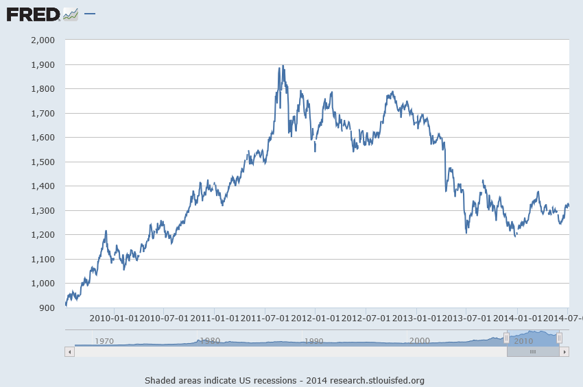
Now the price series shown in the graph above is a random walk, according to auto.arima(.).

In other words, the routine indicates that the optimal model is ARIMA(0,1,0), which is to say that after differencing the price series once, the program suggests the series reduces to a series of independent random values. The automatic exponential smoothing routine in Forecast is ets(.). Running this confirms that simple exponential smoothing, with a smoothing parameter close to 1, is the optimal model – again, consistent with a random walk.

Here’s a graph of these first differences.

1stdiffgold

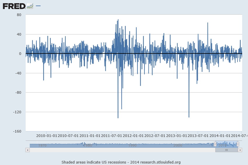
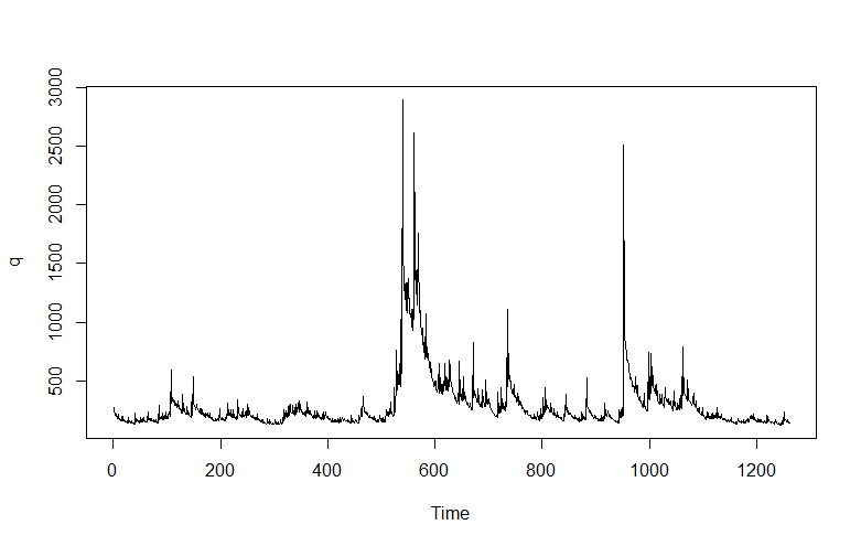
But wait, there is a clustering of volatility of these first differences, which can be accentuated if we square these values, producing the following graph.

volatilityGP

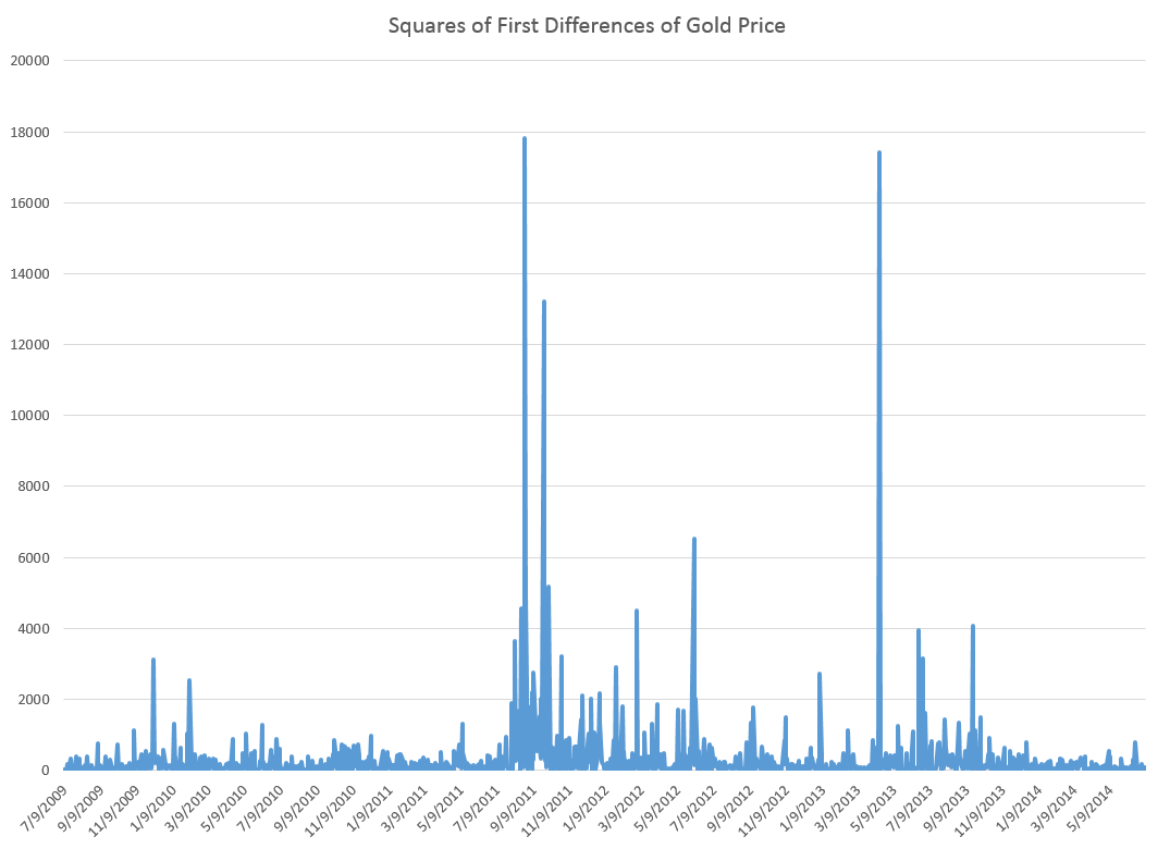
Now in a more or less textbook example, auto.arima(.) develops the following ARIMA model for this series

model

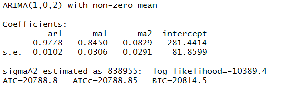
Thus, this estimate of the volatility of the first differences of gold price is modeled as a first order autoregressive process with two moving average terms.

Here is the plot of the fitted values.

Rplot1

Nice.

But of course, we are interested in forecasting, and the results here are somewhat more disappointing.

Basically, this type of model makes a horizontal line prediction at a certain level, which is higher when the past values have been higher.

This is what people in quantitative finance call “persistence” but of course sometimes new things happen, and then these types of models do not do well.

From my research on the volatility literature, it seems that short period forecasts are better than longer period forecasts. Ideally, you update your volatility model daily or at even higher frequencies, and it’s likely your one or two period ahead (minutes, hours, a day) will be more accurate.

Incidentally, exponential smoothing in this context appears to be a total fail, again suggesting this series is a simple random walk.

Recapitulation

There is more here than meets the eye.

First, the auto.arima(.) routines in the Hyndman R Forecast package do a competent job of modeling the clustering of higher first differences of the gold price series here. But, at the same time, they highlight a methodological point. The gold price series really has nonlinear aspects that are not adequately commanded by a purely linear model. So, as in many approximations, the assumption of linearity gets us some part of the way, but deeper analysis indicates the existence of nonlinearities. Kind of interesting.

Of course, I have not told you about the notation ARIMA(p,d,q). Well, p stands for the order of the autoregressive terms in the equation, q stands for the moving average terms, and d indicates the times the series is differenced to reduce it to a stationary time series. Take a look at Forecasting: principles and practice – the free forecasting text of Hyndman and Athanasopoulos – in the chapter on ARIMA modeling for more details.

Incidentally, I think it is great that Hyndman and some of his collaborators are providing an open source, indeed free, forecasting package with automatic forecasting capabilities, along with a high quality and, again, free textbook on forecasting to back it up. Eventually, some of these techniques might get dispersed into the general social environment, potentially raising the level of some discussions and thinking about our common future.

And I guess also I have to say that, ultimately, you need to learn the underlying theory and struggle with the algebra some. It can improve one’s ability to model these series.

Business Forecasting – Some Thoughts About Scope

In many business applications, forecasting is not a hugely complex business. For a sales forecasting, the main challenge can be obtaining the data, which may require sifting through databases compiled before and after mergers or other reorganizations. Often, available historical data goes back only three or four years, before which time product cycles make comparisons iffy. Then, typically, you plug the sales data into an automatic forecasting program, one that can assess potential seasonality, and probably employing some type of exponential smoothing, and, bang, you produce forecasts for one to several quarters going forward.

The situation becomes more complex when you take into account various drivers and triggers for sales. The customer revenues and income are major drivers, which lead into assessments of business conditions generally. Maybe you want to evaluate the chances of a major change in government policy or the legal framework – both which are classifiable under “triggers.” What if the Federal Reserve starts raising the interest rates, for example.

For many applications, a driver-trigger matrix can be useful. This is a qualitative tool for presentations to management. Essentially, it helps keep track of assumptions about the scenarios which you expect to unfold from which you can glean directions of change for the drivers – GDP, interest rates, market conditions. You list the major influences on sales in the first column. In the second column you indicate the direction of this influences (+/-) and in the third column you put in the expected direction of change, plus, minus, or no change.

The next step up in terms of complexity is to collect historical data on the drivers and triggers – “explanatory variables” driving sales in the company. This opens the way for a full-blown multivariate model of sales performance. The hitch is to make this operational, you have to forecast the explanatory variables. Usually, this is done by relying, again, on forecasts by other organizations, such as market research vendors, consensus forecasts such as available from the Survey of Professional Forecasters and so forth. Sometimes it is possible to identify “leading indicators” which can be built into multivariate models. This is really the best of all possible worlds, since you can plug in known values of drivers and get a prediction for the target variable.

The value of forecasting to a business is linked with benefits of improvements in accuracy, as well as providing a platform to explore “what-if’s,” supporting learning about the business, customers, and so forth.

With close analysis, it is often possible to improve the accuracy of sales forecasts by a few percentage points. This may not sound like much, but in a business with $100 million or more in sales, competent forecasting can pay for itself several times over in terms of better inventory management and purchasing, customer satisfaction, and deployment of resources.

Time Horizon

When you get a forecasting assignment, you soon learn about several different time horizons. To some extent, each forecasting time horizon is best approached with certain methods and has different uses.

Conventionally, there are short, medium, and long term forecasting horizons.

In general business applications, the medium term perspective of a few quarters to a year or two is probably the first place forecasting is deployed. The issue is usually the budget, and allocating resources in the organization generally. Exponential smoothing, possibly combined with information about anticipated changes in key drivers, usually works well in this context. Forecast accuracy is a real consideration, since retrospectives on the budget are a common practice. How did we do last year? What mistakes were made? How can we do better?

The longer term forecast horizons of several years or more usually support planning, investment evaluation, business strategy. The M-competitions suggest the issue has to be being able to pose and answer various “what-if’s,” rather than achieving a high degree of accuracy. Of course, I refer here to the finding that forecast accuracy almost always deteriorates in direct proportion to the length of the forecast horizon.

Short term forecasting of days, weeks, a few months is an interesting application. Usually, there is an operational focus. Very short term forecasting in terms of minutes, hours, days is almost strictly a matter of adjusting a system, such as generating electric power from a variety of sources, i.e. combining hydro and gas fired turbines, etc.

As far as techniques, short term forecasting can get sophisticated and mathematically complex. If you are developing a model for minute-by-minute optimization of a system, you may have several months or even years of data at your disposal. There are, thus, more than a half a million minutes in a year.

Forecasting and Executive Decisions

The longer the forecasting horizon, the more the forecasting function becomes simply to “inform judgment.”

A smart policy for an executive is to look at several forecasts, consider several sources of information, before determining a policy or course of action. Management brings judgment to bear on the numbers. It’s probably not smart to just take the numbers on blind faith. Usually, executives, if they pay attention to a presentation, will insist on a coherent story behind the model and the findings, and also checking the accuracy of some points. Numbers need to compute. Round-off-errors need to be buried for purposes of the presentation. Everything should add up exactly.

As forecasts are developed for shorter time horizons and more for direct operation control of processes, acceptance and use of the forecast can become more automatic. This also can be risky, since developers constantly have to ask whether the output of the model is reasonable, whether the model is still working with the new data, and so forth.

Shiny New Techniques

The gap between what is theoretically possible in data analysis and what is actually done is probably widening. Companies enthusiastically take up the “Big Data” mantra – hiring “Chief Data Scientists.” I noticed with amusement an article in a trade magazine quoting an executive who wondered whether hiring a data scientist was something like hiring a unicorn.

There is a lot of data out there, more all the time. More and more data is becoming accessible with expansion of storage capabilities and of course storage in the cloud.

And really the range of new techniques is dazzling.

I’m thinking, for example, of bagging and boosting forecast models. Or of the techniques that can be deployed for the problem of “many predictors,” techniques including principal component analysis, ridge regression, the lasso, and partial least squares.

Probably one of the areas where these new techniques come into their own is in target marketing. Target marketing is kind of a reworking of forecasting. As in forecasting sales generally, you identify key influences (“drivers and triggers”) on the sale of a product, usually against survey data or past data on customers and their purchases. Typically, there is a higher degree of disaggregation, often to the customer level, than in standard forecasting.

When you are able to predict sales to a segment of customers, or to customers with certain characteristics, you then are ready for the sales campaign to this target group. Maybe a pricing decision is involved, or development of a product with a particular mix of features. Advertising, where attitudinal surveys supplement customer demographics and other data, is another key area.

Related Areas

Many of the same techniques, perhaps with minor modifications, are applicable to other areas for what has come to be called “predictive analytics.”

The medical/health field has a growing list of important applications. As this blog tries to show, quantitative techniques, such as logistic regression, have a lot to offer medical diagnostics. I think the extension of predictive analytics to medicine and health care ism at this point, merely a matter of access to the data. This is low-hanging fruit. Physicians diagnosing a guy with an enlarged prostate and certain PSA and other metrics should be able to consult a huge database for similarities with respect to age, health status, collateral medical issues and so forth. There is really no reason to suspect that normally bright, motivated people who progress through medical school and come out to practice should know the patterns in 100,000 medical records of similar cases throughout the nation, or have read all the scientific articles on that particular niche. While there are technical and interpretive issues, I think this corresponds well to what Nate Silver identifies as promising – areas where application of a little quantitative analysis and study can reap huge rewards.

And cancer research is coming to be closely allied with predictive analytics and data science. The paradigmatic application is the DNA assay, where a sample of a tumor is compared with healthy tissue from the same individual to get an idea of what cancer configuration is at play. Indeed, at that fine new day when big pharma will develop hundreds of genetically targeted therapies for people with a certain genetic makeup with a certain cancer – when that wonderful new day comes – cancer treatment may indeed go hand in hand with mathematical analysis of the patient’s makeup.

The Loebner Prize and Turing Test

In a brilliant, early article on whether machines can “think,” Alan Turing, the genius behind a lot of early computer science, suggested that if a machine cannot be distinguished from a human during text-based conversation, that machine could be said to be thinking and have intelligence.

Every year, the Loebner Prize holds this type of Turing comptition. Judges, such as those below, interact with computer programs (and real people posing as computer programs). If a

judges

computer program fools enough people, the program is elible for various prizes.

The 2013 prize was won by Mitsuki Chatbox advertised as an artificial lifeform living on the web.

chatbot

She certainly is fun, and is an avatar of a whole range of chatbots which are increasingly employed in customer service and other business applications.

Mitsuku’s botmaster, Steve Worswick, ran a music website with a chatbot. Apparently, more people visited to chat than for music so he concentrated his efforts on the bot, which he still regards as a hobby. Mitsuku uses AIML (Artificial Intelligence Markup Language) used by members of pandorabot.

Mitsuki is very cute, which perhaps one reason why she gets worldwide attention.

pageviews

It would be fun to develop a forecastbot, capable of answering basic questions about which forecasting method might be appropriate. We’ve all seen those flowcharts and tabular arrays with data characteristics and forecast objectives on one side, and recommended methods on the other.


Data Analytics Reverses Grandiose Claims for California’s Monterey Shale Formation

In May, “federal officials” contacted the Los Angeles Times with advance news of a radical revision of estimates of reserves in the Monterey Formation,

Just 600 million barrels of oil can be extracted with existing technology, far below the 13.7 billion barrels once thought recoverable from the jumbled layers of subterranean rock spread across much of Central California, the U.S. Energy Information Administration said.

The LA Times continues with a bizarre story of how “an independent firm under contract with the government” made the mistake of assuming that deposits in the Monterey Shale formation were as easily recoverable as those found in shale formations elsewhere.

There was a lot more too, such as the information that –

The Monterey Shale formation contains about two-thirds of the nation’s shale oil reserves. It had been seen as an enormous bonanza, reducing the nation’s need for foreign oil imports through the use of the latest in extraction techniques, including acid treatments, horizontal drilling and fracking…

The estimate touched off a speculation boom among oil companies.

Well, I’ve combed the web trying to find more about this “mistake,” deciding that, probably, it was the analysis of David Hughes in “Drilling California,” released in March of this year, that turned the trick.

Hughes – a geoscientist working decades with the Geological Survey of Canada – utterly demolishes studies which project 15 billion barrels in reserve in the Monterey Formation. And he does this by analyzing an extensive database (Big Data) of wells drilled in the Formation.

The video below is well worth the twenty minutes or so. It’s a tour de force of data analysis, but it takes a little patience at points.

First, though, check out a sample of the hype associated with all this, before the overblown estimates were retracted.

Monterey Shale: California’s Trillion-Dollar Energy Source

Here’s a video on Hughes’ research in Drilling California

Finally, here’s the head of the US Energy Information Agency in December 2013, discussing a preliminary release of figures in the 2014 Energy Outlook, also released in May 2014.

Natural Gas 2014 Projections by the EIA’s Adam Sieminski

One question is whether the EIA projections eventually will be acknowledged to be affected by a revision of reserves for a formation that is thought to contain two thirds of all shale oil in the US.

Some Ways in Which Bayesian Methods Differ From the “Frequentist” Approach

I’ve been doing a deep dive into Bayesian materials, the past few days. I’ve tried this before, but I seem to be making more headway this time.

One question is whether Bayesian methods and statistics informed by the more familiar frequency interpretation of probability can give different answers.

I found this question on CrossValidated, too – Examples of Bayesian and frequentist approach giving different answers.

Among other things, responders cite YouTube videos of John Kruschke – the author of Doing Bayesian Data Analysis A Tutorial With R and BUGS

Here is Kruschke’s “Bayesian Estimation Supercedes the t Test,” which, frankly, I recommend you click on after reading the subsequent comments here.

I guess my concern is not just whether Bayesian and the more familiar frequentist methods give different answers, but, really, whether they give different predictions that can be checked.

I get the sense that Kruschke focuses on the logic and coherence of Bayesian methods in a context where standard statistics may fall short.

But I have found a context where there are clear differences in predictive outcomes between frequentist and Bayesian methods.

This concerns Bayesian versus what you might call classical regression.

In lecture notes for a course on Machine Learning given at Ohio State in 2012, Brian Kulis demonstrates something I had heard mention of two or three years ago, and another result which surprises me big-time.

Let me just state this result directly, then go into some of the mathematical details briefly.

Suppose you have a standard ordinary least squares (OLS) linear regression, which might look like,

linreg

where we can assume the data for y and x are mean centered. Then, as is well, known, assuming the error process ε is N(0,σ) and a few other things, the BLUE (best linear unbiased estimate) of the regression parameters w is –

regressionformulaNow Bayesian methods take advantage of Bayes Theorem, which has a likelihood function and a prior probability on the right hand side of the equation, and the resulting posterior distribution on the left hand side of the equation.

What priors do we use for linear regression in a Bayesian approach?

Well, apparently, there are two options.

First, suppose we adopt priors for the predictors x, and suppose the prior is a normal distribution – that is the predictors are assumed to be normally distributed variables with various means and standard deviations.

In this case, amazingly, the posterior distribution for a Bayesian setup basically gives the equation for ridge regression.

ridgebayes

On the other hand, assuming a prior which is a Laplace distribution gives a posterior distribution which is equivalent to the lasso.

This is quite stunning, really.

Obviously, then, predictions from an OLS regression, in general, will be different from predictions from a ridge regression estimated on the same data, depending on the value of the tuning parameter λ (See the post here on this).

Similarly with a lasso regression – different forecasts are highly likely.

Now it’s interesting to question which might be more accurate – the standard OLS or the Bayesian formulations. The answer, of course, is that there is a tradeoff between bias and variability effected here. In some situations, ridge regression or the lasso will produce superior forecasts, measured, for example, by root mean square error (RMSE).

This is all pretty wonkish, I realize. But it conclusively shows that there can be significant differences in regression forecasts between the Bayesian and frequentist approaches.

What interests me more, though, is Bayesian methods for forecast combination. I am still working on examples of these procedures. But this is an important area, and there are a number of studies which show gains in forecast accuracy, measured by conventional metrics, for Bayesian model combinations.

Predicting Season Batting Averages, Bernoulli Processes – Bayesian vs Frequentist

Recently, Nate Silver boosted Bayesian methods in his popular book The Signal and the Noise – Why So Many Predictions Fail – But Some Don’t. I’m guessing the core application for Silver is estimating batting averages. Silver first became famous with PECOTA, a system for forecasting the performance of Major League baseball players.

Let’s assume a player’s probability p of getting a hit is constant over a season, but that it varies from year to year. He has up years, and down years. And let’s compare frequentist (gnarly word) and Bayesian approaches at the beginning of the season.

The frequentist approach is based on maximum likelihood estimation with the binomial formula

binomial

Here the n and the k in parentheses at the beginning of the expression stand for the combination of n things taken k at a time. That is, the number of possible ways of interposing k successes (hits) in n trials (times at bat) is the combination of n things taken k at a time (formula here).

If p is the player’s probability of hitting at bat, then the entire expression is the probability the player will have k hits in n times at bat.

The Frequentist Approach

There are a couple of ways to explain the frequentist perspective.

One is that this binomial expression is approximated to a higher and higher degree of accuracy by a normal distribution. This means that – with large enough n – the ratio of hits to total times at bat is the best estimate of the probability of a player hitting at bat – or k/n.

This solution to the problem also can be shown to follow from maximizing the likelihood of the above expression for any n and k. The large sample or asymptotic and maximum likelihood solutions are numerically identical.

The problem comes with applying this estimate early on in the season. So if the player has a couple of rough times at bat initially, the frequentist estimate of his batting average for the season at that point is zero.

The Bayesian Approach

The Bayesian approach is based on the posterior probability distribution for the player’s batting average. From Bayes Theorem, this is a product of the likelihood and a prior for the batting average.

Now generally, especially if we are baseball mavens, we have an idea of player X’s batting average. Say we believe it will be .34 – he’s going to have a great season, and did last year.

In this case, we can build that belief or information into a prior that is a beta distribution with two parameters α and β that generate a mean of α/(α+β).

In combination with the binomial likelihood function, this beta distribution prior combines algebraically into a closed form expression for another beta function with parameters which are adjusted by the values of k and n-k (the number of strike-outs). Note that walks (also being hit by the ball) do not count as times at bat.

This beta function posterior distribution then can be moved back to the other side of the Bayes equation when there is new information – another hit or strikeout.

Taking the average of the beta posterior as the best estimate of p, then, we get successive approximations, such as shown in the following graph.

BAyesbatting

So the player starts out really banging ‘em, and the frequentist estimate of his batting average for that season starts at 100 percent. The Bayesian estimate on the other hand is conditioned by a belief that his batting average should be somewhere around 0.34. In fact, as the grey line indicates, his actual probability p for that year is 0.3. Both the frequentist and Bayesian estimates converge towards this value with enough times at bat.

I used α=33 and β=55 for the initial values of the Beta distribution.

See this for a great discussion of the intuition behind the Beta distribution.

This, then, is a worked example showing how Bayesian methods can include prior information, and have small sample properties which can outperform a frequentist approach.

Of course, in setting up this example in a spreadsheet, it is possible to go on and generate a large number of examples to explore just how often the Bayesian estimate beats the frequentist estimate in the early part of a Bernoulli process.

Which goes to show that what you might call the classical statistical approach – emphasizing large sample properties, covering all cases, still has legs.

Bayesian Methods in Forecasting and Data Analysis

The basic idea of Bayesian methods is outstanding. Here is a way of incorporating prior information into analysis, helping to manage, for example, small samples that are endemic in business forecasting.

What I am looking for, in the coming posts on this topic, is what difference does it make.

Bayes Theorem

Just to set the stage, consider the simple statement and derivation of Bayes Theorem –

BayesThm

Here A and B are events or occurrences, and P(.) is the probability (of the argument . ) function. So P(A) is the probability of event A. And P(A|B) is the conditional probability of event A, given that event B has occurred.

A Venn diagram helps.

Venn

Here, there is the universal set U, and the two subsets A and B. The diagram maps some type of event or belief space. So the probability of A or P(A) is the ratio of the areas A and U.

Then, the conditional probability of the occurrence of A, given the occurrence of B is the ratio of the area labeled AB to the area labeled B in the diagram. Also area AB is the intersection of the areas A and B or A ∩ B in set theory notation. So we have P(A|B)=P(A ∩ B)/P(B).

By the same logic, we can create the expression for P(B|A) = P(B ∩ A)/P(A).

Now to be mathematically complete here, we note that intersection in set theory is commutative, so A ∩ B = B ∩ A, and thus P(A ∩ B)=P(B|A)•P(A). This leads to the initially posed formulation of Bayes Theorem by substitution.

So Bayes Theorem, in its simplest terms, follows from the concept or definition of conditional probability – nothing more.

Prior and Posterior Distributions and the Likelihood Function

With just this simple formulation, one can address questions that are essentially what I call “urn problems.” That is, having drawn some number of balls of different colors from one of several sources (urns), what is the probability that the combination of, say, red and white balls drawn comes from, say, Urn 2? Some versions of even this simple setup seem to provide counter-intuitive values for the resulting P(A|B).

But I am interested primarily in forecasting and data analysis, so let me jump ahead to address a key interpretation of the Bayes Theorem.

Thus, what is all this business about prior and posterior distributions, and also the likelihood function?

Well, considering Bayes Theorem as a statement of beliefs or subjective probabilities, P(A) is the prior distribution, and P(A|B) is the posterior distribution, or the probability distribution that follows revelation of the facts surrounding event (or group of events) B.

P(B|A) then is the likelihood function.

Now all this is more understandable, perhaps, if we reframe Bayes rule in terms of data y and parameters θ of some statistical model.

So we have

Bayes2

In this case, we have some data observations {y1, y2,…,yn}, and can have covariates x={x1,..,xk}, which could be inserted in the conditional probability of the data, given the parameters on the right hand side of the equation, as P(y|θ,x).

In any case, clear distinctions between the Bayesian and frequentist approach can be drawn with respect to the likelihood function P(y|θ).

So the frequentist approach focuses on maximizing the likelihood function with respect to the unknown parameters θ, which of course can be a vector of several parameters.

As one very clear overview says,

One maximizes the likelihood function L(·) with respect the parameters to obtain the maximum likelihood estimates; i.e., the parameter values most likely to have produced the observed data. To perform inference about the parameters, the frequentist recognizes that the estimated parameters ˆ result from a single sample, and uses the sampling distribution to compute standard errors, perform hypothesis tests, construct confidence intervals, and the like..

In the Bayesian perspective, the unknown parameters θ are treated as random variables, while the observations y are treated as fixed in some sense.

The focus of attention is then on how the observed data y changes the prior distribution P(θ) into the posterior distribution P(y|θ).

The posterior distribution, in essence, translates the likelihood function into a proper probability distribution over the unknown parameters, which can be summarized just as any probability distribution; by computing expected values, standard deviations, quantiles, and the like. What makes this possible is the formal inclusion of prior information in the analysis.

One difference then is that the frequentist approach optimizes the likelihood function with respect to the unknown parameters, while the Bayesian approach is more concerned with integrating the posterior distribution to obtain values for key metrics and parameters of the situation, after data vector y is taken into account.

Extracting Parameters From the Posterior Distribution

The posterior distribution, in other words, summarizes the statistical model of a phenomenon which we are analyzing, given all the available information.

That sounds pretty good, but the issue is that the result of all these multiplications and divisions on the right hand side of the equation can lead to a posterior distribution which is difficult to evaluate. It’s a probability distribution, for example, and thus some type of integral equation, but there may be no closed form solution.

Prior to Big Data and the muscle of modern computer computations, Bayesian statisticians spent a lot of time and energy searching out conjugate prior’s. Wikipedia has a whole list of these.

So the Beta distribution is a conjugate prior for a Bernoulli distribution – the familiar probability p of success and probability q of failure model (like coin-flipping, when p=q=0.5). This means simply that multiplying a Bernoulli likelihood function by an appropriate Beta distribution leads to a posterior distribution that is again a Beta distribution, and which can be integrated and, also, which supports a sort of loop of estimation with existing and then further data.

Here’s an example and prepare yourself for the flurry of symbolism –

BayesexampleB

Note the update of the distribution of whether the referendum is won or lost results in a much sharper distribution and increase in the probability of loss of the referendum.

Monte Carlo Methods

Stanislaus Ulam, along with John von Neumann, developed Monte Carlo simulation methods to address what might happen if radioactive materials were brought together in sufficient quantities and with sufficient emissions of neutrons to achieve a critical mass. That is, researchers at Los Alamos at the time were not willing to simply experiment to achieve this effect, and watch the unfolding.

Monte Carlo computation methods, thus, take complicated mathematical relationships and calculate final states or results from random assignments of values of the explanatory variables.

Two algorithms—the Gibbs sampling and Metropolis-Hastings algorithms— are widely used for applied Bayesian work, and both are Markov chain Monte Carlo methods.

The Markov chain aspect of the sampling involves selection of the simulated values along a path determined by prior values that have been sampled.

The object is to converge on the key areas of the posterior distribution.

The Bottom Line

It has taken me several years to comfortably grasp what is going on here with Bayesian statistics.

The question, again, is what difference does it make in forecasting and data analysis? And, also, if it made a difference in comparison with a frequentist interpretation or approach, would that be an entirely good thing?

A lot of it has to do with a reorientation of perspective. So some of the enthusiasm and combative qualities of Bayesians seems to come from their belief that their system of concepts is simply the only coherent one.

But there are a lot of medical applications, including some relating to trials of new drugs and procedures. What goes there? Is the representation that it is not necessary to take all this time required by the FDA to test a drug or procedure, when we can access prior knowledge and bring it to the table in evaluating outcomes?

Or what about forecasting applications? Is there something more productive about some Bayesian approaches to forecasting – something that can be measured in, for example, holdout samples or the like? Or I don’t know whether that violates the spirit of the approach – holdout samples.

I’m planning some posts on this topic. Let me know what you think.

Top picture from Los Alamos laboratories

Jobs and the Next Wave of Computerization

A duo of researchers from Oxford University (Frey and Osborne) made a splash with their analysis of employment and computerization in the US (English spelling). Their research, released September of last year, projects that –

47 percent of total US employment is in the high risk category, meaning that associated occupations are potentially automatable over some unspecified number of years, perhaps a decade or two..

Based on US Bureau of Labor Statistics (BLS) classifications from O*NET Online, their model predicts that most workers in transportation and logistics occupations, together with the bulk of office and administrative support workers, and labour in production occupations, are at risk.

This research deserves attention, if for no other reason than masterful discussions of the impact of technology on employment and many specific examples of new areas for computerization and automation.

For example, I did not know,

Oncologists at Memorial Sloan-Kettering Cancer Center are, for example, using IBM’s Watson computer to provide chronic care and cancer treatment diagnostics. Knowledge from 600,000 medical evidence reports, 1.5 million patient records and clinical trials, and two million pages of text from medical journals, are used for benchmarking and pattern recognition purposes. This allows the computer to compare each patient’s individual symptoms, genetics, family and medication history, etc., to diagnose and develop a treatment plan with the highest probability of success..

There are also specifics of computerized condition monitoring and novelty detection -substituting for closed-circuit TV operators, workers examining equipment defects, and clinical staff in intensive care units.

A followup Atlantic Monthly article – What Jobs Will the Robots Take? – writes,

We might be on the edge of a breakthrough moment in robotics and artificial intelligence. Although the past 30 years have hollowed out the middle, high- and low-skill jobs have actually increased, as if protected from the invading armies of robots by their own moats. Higher-skill workers have been protected by a kind of social-intelligence moat. Computers are historically good at executing routines, but they’re bad at finding patterns, communicating with people, and making decisions, which is what managers are paid to do. This is why some people think managers are, for the moment, one of the largest categories immune to the rushing wave of AI.

Meanwhile, lower-skill workers have been protected by the Moravec moat. Hans Moravec was a futurist who pointed out that machine technology mimicked a savant infant: Machines could do long math equations instantly and beat anybody in chess, but they can’t answer a simple question or walk up a flight of stairs. As a result, menial work done by people without much education (like home health care workers, or fast-food attendants) have been spared, too.

What Frey and Osborne at Oxford suggest is an inflection point, where machine learning (ML) and what they call mobile robotics (MR) have advanced to the point where new areas for applications will open up – including a lot of menial, service tasks that were not sufficiently routinized for the first wave.

In addition, artificial intelligence (AI) and Big Data algorithms are prying open up areas formerly dominated by intellectual workers.

The Atlantic Monthly article cited above has an interesting graphic –

jobsautomationSo at the top of this chart are the jobs which are at 100 percent risk of being automated, while at the bottom are jobs which probably will never be automated (although I do think counseling can be done to a certain degree by AI applications).

The Final Frontier

This blog focuses on many of the relevant techniques in machine learning – basically unsupervised learning of patterns – which in the future will change everything.

Driverless cars are the wow example, of course.

Bottlenecks to moving further up the curve of computerization are highlighted in the following table from the Oxford U report.

ONETvars

As far as dexterity and flexibility goes, Baxter shows great promise, as the following YouTube from his innovators illustrates.

There also are some wonderful examples of apparent creativity by computers or automatic systems, which I plan to detail in a future post.

Frey and Osborn, reflecting on their research in a 2014 discussion, conclude

So, if a computer can drive better than you, respond to requests as well as you and track down information better than you, what tasks will be left for labour? Our research suggests that human social intelligence and creativity are the domains were labour will still have a comparative advantage. Not least, because these are domains where computers complement our abilities rather than substitute for them. This is because creativity and social intelligence is embedded in human values, meaning that computers would not only have to become better, but also increasingly human, to substitute for labour performing such work.

Our findings thus imply that as technology races ahead, low-skill workers will need to reallocate to tasks that are non-susceptible to computerisation – i.e., tasks requiring creative and social intelligence. For workers to win the race, however, they will have to acquire creative and social skills. Development strategies thus ought to leverage the complementarity between computer capital and creativity by helping workers transition into new work, involving working with computers and creative and social ways.

Specifically, we recommend investing in transferable computer-related skills that are not particular to specific businesses or industries. Examples of such skills are computer programming and statistical modeling. These skills are used in a wide range of industries and occupations, spanning from the financial sector, to business services and ICT.

Implications For Business Forecasting

People specializing in forecasting for enterprise level business have some responsibility to “get ahead of the curve” – conceptually, at least.

Not everybody feels comfortable doing this, I realize.

However, I’m coming to the realization that these discussions of how many jobs are susceptible to “automation” or whatever you want to call it (not to mention jobs at risk for “offshoring”) – these discussions are really kind of the canary in the coal mine.

Something is definitely going on here.

But what are the metrics? Can you backdate the analysis Frey and Osborne offer, for example, to account for the coupling of productivity growth and slower employment gains since the last recession?

Getting a handle on this dynamic in the US, Europe, and even China has huge implications for marketing, and, indeed, social control.

Machine Learning and Next Week

Here is a nice list of machine learning algorithms. Remember, too, that they come in two or three flavors – supervised, unsupervised, semi-supervised, and reinforcement learning.

MachineLearning

An objective of mine is to cover each of these techniques with an example or two, with special reference to their relevance to forecasting.

I got this list, incidentally, from an interesting Australian blog Machine Learning Mastery.

The Coming Week

Aligned with this marvelous list, I’ve decided to focus on robotics for a few blog posts coming up.

This is definitely exploratory, but recently I heard a presentation by an economist from the National Association of Manufacturers (NAM) on manufacturing productivity, among other topics. Apparently, robotics is definitely happening on the shop floor – especially in the automobile industry, but also in semiconductors and electronics assembly.

And, as mankind pushes the envelope, drilling for oil in deeper and deeper areas offshore and handling more and more radioactive and toxic material, the need for significant robotic assistance is definitely growing.

I’m looking for indices and how to construct them – how to guage the line between merely automatic and what we might more properly call robotic.

LInks – late May

US and Global Economic Prospects

Goldman’s Hatzius: Rationale for Economic Acceleration Is Intact

We currently estimate that real GDP fell -0.7% (annualized) in the first quarter, versus a December consensus estimate of +2½%. On the face of it, this is a large disappointment. It raises the question whether 2014 will be yet another year when initially high hopes for growth are ultimately dashed.

 Today we therefore ask whether our forecast that 2014-2015 will show a meaningful pickup in growth relative to the first four years of the recovery is still on track. Our answer, broadly, is yes. Although the weak first quarter is likely to hold down real GDP for 2014 as a whole, the underlying trends in economic activity are still pointing to significant improvement….

 The basic rationale for our acceleration forecast of late 2013 was twofold—(1) an end to the fiscal drag that had weighed on growth so heavily in 2013 and (2) a positive impulse from the private sector following the completion of the balance sheet adjustments specifically among US households. Both of these points remain intact.

Economy and Housing Market Projected to Grow in 2015

Despite many beginning-of-the-year predictions about spring growth in the housing market falling flat, and despite a still chugging economy that changes its mind quarter-to-quarter, economists at the National Association of Realtors and other industry groups expect an uptick in the economy and housing market through next year.

The key to the NAR’s optimism, as expressed by the organization’s chief economist, Lawrence Yun, earlier this week, is a hefty pent-up demand for houses coupled with expectations of job growth—which itself has been more feeble than anticipated. “When you look at the jobs-to-population ratio, the current period is weaker than it was from the late 1990s through 2007,” Yun said. “This explains why Main Street America does not fully feel the recovery.”

Yun’s comments echo those in a report released Thursday by Fitch Ratings and Oxford Analytica that looks at the unusual pattern of recovery the U.S. is facing in the wake of its latest major recession. However, although the U.S. GDP and overall economy have occasionally fluctuated quarter-to-quarter these past few years, Yun said that there are no fresh signs of recession for Q2, which could grow about 3 percent.

Report: San Francisco has worse income inequality than Rwanda

If San Francisco was a country, it would rank as the 20th most unequal nation on Earth, according to the World Bank’s measurements.

Googlebus

Climate Change

When Will Coastal Property Values Crash And Will Climate Science Deniers Be The Only Buyers?

sea

How Much Will It Cost to Solve Climate Change?

Switching from fossil fuels to low-carbon sources of energy will cost $44 trillion between now and 2050, according to a report released this week by the International Energy Agency.

Natural Gas and Fracking

How The Russia-China Gas Deal Hurts U.S. Liquid Natural Gas Industry

This could dampen the demand – and ultimately the price for – LNG from the United States. East Asia represents the most prized market for producers of LNG. That’s because it is home to the top three importers of LNG in the world: Japan, South Korea and China. Together, the three countries account for more than half of LNG demand worldwide. As a result, prices for LNG are as much as four to five times higher in Asia compared to what natural gas is sold for in the United States.

The Russia-China deal may change that.

If LNG prices in Asia come down from their recent highs, the most expensive LNG projects may no longer be profitable. That could force out several of the U.S. LNG projects waiting for U.S. Department of Energy approval. As of April, DOE had approved seven LNG terminals, but many more are waiting for permits.

LNG terminals in the United States will also not be the least expensive producers. The construction of several liquefaction facilities in Australia is way ahead of competitors in the U.S., and the country plans on nearly quadrupling its LNG capacity by 2017. More supplies and lower-than-expected demand from China could bring down prices over the next several years.

Write-down of two-thirds of US shale oil explodes fracking mythThis is big!

Next month, the US Energy Information Administration (EIA) will publish a new estimate of US shale deposits set to deal a death-blow to industry hype about a new golden era of US energy independence by fracking unconventional oil and gas.

EIA officials told the Los Angeles Times that previous estimates of recoverable oil in the Monterey shale reserves in California of about 15.4 billion barrels were vastly overstated. The revised estimate, they said, will slash this amount by 96% to a puny 600 million barrels of oil.

The Monterey formation, previously believed to contain more than double the amount of oil estimated at the Bakken shale in North Dakota, and five times larger than the Eagle Ford shale in South Texas, was slated to add up to 2.8 million jobs by 2020 and boost government tax revenues by $24.6 billion a year.

China

The Annotated History Of The World’s Next Reserve Currency

yuanhistory

Goldman: Prepare for Chinese property bust

…With demand poised to slow given a tepid economic backdrop, weaker household affordability, rising mortgage rates and developer cash flow weakness, we believe current construction capacity of the domestic property industry may be excessive. We estimate an inventory adjustment cycle of two years for developers, driving 10%-15% price cuts in most cities with 15% volume contraction from 2013 levels in 2014E-15E. We also expect M&A activities to take place actively, favoring developers with strong balance sheet and cash flow discipline.

China’s Shadow Banking Sector Valued At 80% of GDP

The China Banking Regulatory Commission has shed light on the country’s opaque shadow banking sector. It was as large as 33 trillion yuan ($5.29 trillion) in mid-2013 and equivalent to 80% of last year’s GDP, according to Yan Qingmin, a vice chairman of the commission.

In a Tuesday WeChat blog sent by the Chong Yang Institute for Financial Studies, Renmin University, Yan wrote that his calculation is based on shadow lending activities from asset management businesses to trust companies, a definition he said was very broad.  Yan said the rapid expansion of the sector, which was equivalent to 53% of GDP in 2012, entailed risks of some parts of the shadow banking business, but not necessarily the Chinese economy.

Yan’s estimation is notably higher than that of the Chinese Academy of Social Sciences. The government think tank said on May 9 that the sector has reached 27 trillion yuan ($4.4 trillion in 2013) and is equivalent to nearly one fifth of the domestic banking sector’s total assets.

Massive, Curvaceous Buildings Designed to Imitate a Mountain Forest

Chinamassive

Information Technology (IT)

I am an IT generalist. Am I doomed to low pay forever? Interesting comments and suggestions to this question on a Forum maintained by The Register.

I’m an IT generalist. I know a bit of everything – I can behave appropriately up to Cxx level both internally and with clients, and I’m happy to crawl under a desk to plug in network cables. I know a little bit about how nearly everything works – enough to fill in the gaps quickly: I didn’t know any C# a year ago, but 2 days into a project using it I could see the offshore guys were writing absolute rubbish. I can talk to DB folks about their DBs; network guys about their switches and wireless networks; programmers about their code and architects about their designs. Don’t get me wrong, I can do as well as talk, programming, design, architecture – but I would never claim to be the equal of a specialist (although some of the work I have seen from the soi-disant specialists makes me wonder whether I’m missing a trick).

My principle skill, if there is one – is problem resolution, from nitty gritty tech details (performance and functionality) to handling tricky internal politics to detoxify projects and get them moving again.

How on earth do I sell this to an employer as a full-timer or contractor? Am I doomed to a low income role whilst the specialists command the big day rates? Or should I give up on IT altogether

Crowdfunding is brutal… even when it works

China bans Windows 8

China has banned government use of Windows 8, Microsoft Corp’s latest operating system, a blow to a US technology company that has long struggled with sales in the country.

The Central Government Procurement Center issued the ban on installing Windows 8 on Chinese government computers as part of a notice on the use of energy-saving products, posted on its website last week.

Data Analytics

Statistics of election irregularities – good forensic data analytics.