Tag Archives: Global Business Forecasts

Negative Nominal Interest Rates – the European Central Bank Experiment

Larry Summers, former US Treasury Secretary and, earlier, President of Harvard delivered a curious speech at an IMF Economic Forum last year. After nice words about Stanley Fischer, currently Vice Chair of the Fed, Summers entertains the notion of negative interest rates to combat secular stagnation and restore balance between aggregate demand and supply at something like full employment.

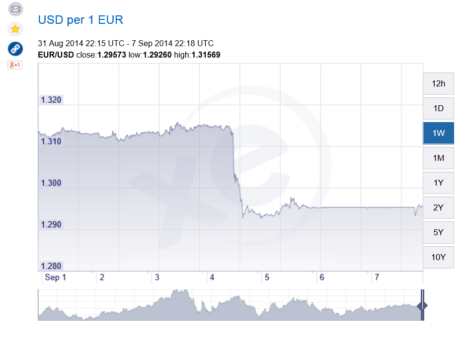
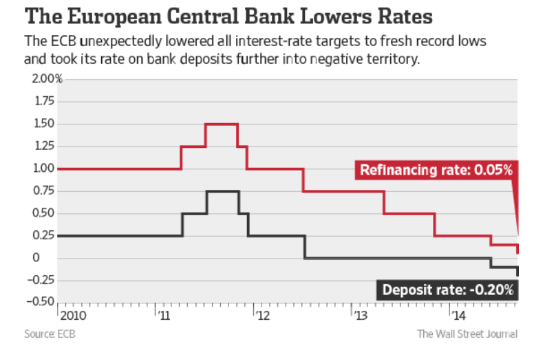
Fast forward to June 2014, when the European Central Bank (ECB) pushes the interest rate on deposits European banks hold in the ECB into negative territory. And on September 4, the ECB drops the deposit rates further to -0.2 percent, also reducing a refinancing rate to virtually zero.

ECBnegint

The ECB discusses this on its website – Why Has the ECB Introduced a Negative interest Rate. After highlighting the ECB mandate to ensure price stability by aiming for an inflation rate of below but close to 2% over the medium term, the website observes euro area inflation is expected to remain considerably below 2% for a prolonged period.

This provides a rationale for lower interest rates, of which there are principally three under ECB control – a marginal lending facility for overnight lending to banks, the main refinancing operations and the deposit facility.

Note that the main refinancing rate is the rate at which banks can regularly borrow from the ECB while the deposit rate is the rate banks receive for funds parked at the central bank.

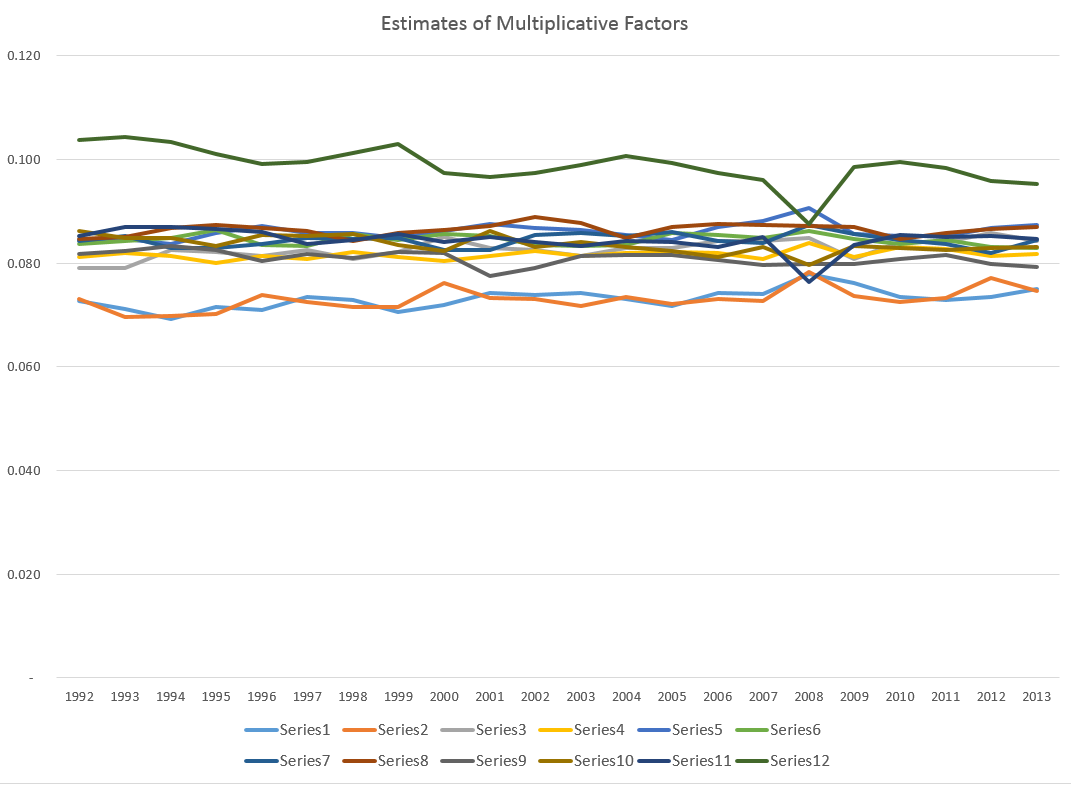
The ECB is adjusting interest rates under their control across the board, as suggested by the chart, but worries that to maintain a functioning money market in which commercial banks lend to each other, these rates cannot be too close to each other.

So, bottom line, the deposit rate was lowered to − 0.10 % in June to maintain this corridor, and then further as the refinancing rate was dropped to -.05 percent.

The hope is that lower refinancing rates will mean lower rates for customers for bank loans, while negative deposit rates will act as a disincentive for banks to simply park excess reserves in the ECB.

Nominal Versus Real Interest Rates and Bond Yields

If you want to prep for, say, negative yields on two year Irish bonds, or issuance of various European bonds with negative yield, as well as the negative yields of a variety of US securities in recent years, after inflation, check out How Low Can You Go? Negative Interest Rates and Investors’ Flight to Safety.

An asset can generate a negative yield, on a conventional, rather than catastrophic basis, in a nominal or real, which is to say, inflation-adjusted, sense.

Some examples of negative real interest rates of yields –

The yield to maturity on the 5-year Treasury note has been below 2 percent since July 2010, and the yield to maturity on the 10-year Treasury note has been below 2 percent since May 2012. Yet, looking forward, the Federal Open Market Committee in January 2012 announced an inflation target of 2 percent—implying an anticipated negative real yield over the life of the securities. Investors, facing uncertainty, appear willing to pay the U.S. government—when measured in real, ex post inflation-adjusted dollars—for the privilege of owning Treasury securities.

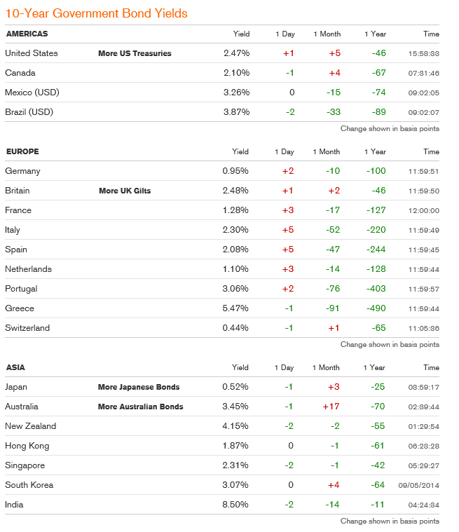
And the current government bond yield situation, from Bloomberg, shows important instances of negative yields, notably Germany and Japan – two of the largest global economies. Click to enlarge.

bondyields

Where the ECB Goes From Here

Mario Draghi, ECB head, gave a speech clearly stating monetary policy is not enough, at the recent Jackson Hole conference of central bankers. After this, the financial press was abuzz with the idea Draghi is moving toward the Japanese leader Abe’s formulation in which there are three weapons or arrows in the Japanese formulation– monetary policy, fiscal policy and structural reforms.

The problem, in the case of the Eurozone, is achieving political consensus for fiscal policies such as backing bonds for badly needed infrastructure development. German opposition seems to be sustained and powerful.

Because of the “political economy” factors , currency and banking problems in the Eurozone are probably more complicated and puzzling than many business executives and managers, looking for a take on the situation, would prefer.

A Thought Experiment

Before diving into this conceptually hazardous topic, though, I’d like to pose a puzzle for readers.

Can banks realistically “charge” negative interest rates to commercial customers?

I seem to have cooked up a spreadsheet where such loans could pay a rate of positive real return to banks, if the rate of deflation can be projected.  In one variant, the bank collects a lending fee at the outset and then the interest rate for installments is negative.

The “save” for banks is that future deflation could inflate the real value of declining nominal installment payments, creating a present value of this stream of payments which is greater than the simple sum of such payments.

I’m not ready for primetime television with this, but it seems such a world encapsulates a very dour view of the future – one that may not be too far from the actual situation in Europe and Japan.

Money black hole at top from Conservative Read

Something is Happening in Europe

Something is going on in Europe.

Take a look at this chart of the euro/dollar exchange rate, and how some event triggered a step down mid week of last week (from xe.com).

euroexchange

The event in question was a press conference by Mario Draghi (See the Wall Street Journal real time blog on this event at Mario Draghi Delivers Fresh ECB Plan — Recap).

The European Central Bank under Draghi is moving into exotic territory – trying negative interest rates on bank deposits and toying with variants of Quantitative Easing (QE) involving ABS – asset backed securities.

All because the basic numbers for major European economies, including notably Germany and France (as well as long-time problem countries such as Spain), are not good. Growth has stalled or is reversing, bank lending is falling, and deflation stalks the European markets.

Europe – which, of course, is sectored into the countries inside and outside the currency union, countries in the common market, and countries in none of the above – accounts for several hundred million persons and maybe 20-30 percent of global production.

So what happens there is significant.

Then there is the Ukraine crisis.

Zerohedge ran this graphic recently showing the dependence of European countries on gas from Russia.

eurdependence

The US-led program of imposing sanctions on Russia – key individuals, companies, banks perhaps – flies in the face of the physical dependence of Germany, for example, on Russian gas.

On the other hand, there is lots of history here on all sides, including, notably, the countries formerly in the USSR in eastern Europe, who no doubt fear the increasingly nationalistic or militant stance shown by Russia currently in, for example, re-acquiring Crimea.

As Chancellor Merkel has stressed, this is an area for diplomacy and negotiation – although there are other voices and forces ready to rush more weapons and even troops to the region of conflict.

Finally, as I have been stressing from time to time, there is an emerging demographic reality which many European nations have to confront.

Edward Hugh has several salient posts on possibly overlooked impacts of aging on the various macroeconomies involved.

There also is the vote on Scotland coming up in the United Kingdom (what we may, if the “yes” votes carry, need to start calling “the British Isles.”)

I’d like to keep current with the signals coming from Europe in a few blogs upcoming – to see, for example, whether swing events in the next six months to a year could originate there.

US Surge in 2nd Quarter GDP

Statistica put together this graphic showing quarter-over-quarter growth in US real GDP from 2009 to the 2nd quarter of 2014.

QoQRGDPGr

The last bar in the chart, showing 4.2 percent growth, is the 2nd quarter 2014 estimate, released by The Bureau of Economic Analysis (BEA) August 28. This represents a slight upward revision from the 4.0 percent “advance estimate” released in July.

Notice these are quarter-over-quarter growth rates, and, as the Statistica chart shows, are fairly volatile.

Thus, a 4.1 percent real or inflation-adjusted growth rate for the April through June 2014 period does not mean 2014 growth will roll in at this rate.

In fact, as the Forbes item on this release highlights,

Dan North, chief economist at Euler Hermes North America… warns GDP watchers should not get too excited…since the economy contracted 2.1% in the first quarter of this year the large jump is payback and in the first half of 2014 the economy gained just 1%. North expects third and fourth quarter GDP to gain around 3% which would round out to an uninspiring roughly 2% growth for the year.

The BEA presents the following detail on the growth estimate (click to enlarge).

BEAtab

Personal consumption expenditures are the largest component in the real GDP series, and bounced back to 2.5 percent growth in the 2nd quarter. Gross private domestic investment surged 17.5 percent for Q2 over Q1, and included healthy 10.7 Q-over-Q growth in investment in equipment. Exports also showed solid Q-over-Q growth.

Europe and Japan

Europe and Japan numbers for the 2nd Quarter are more pessimistic.

Here’s a comparison with European Q-over-Q real growth rates from Eurostat .

eurostat

The EA 18 is the Euro Area, which includes Belgium, Germany, Estonia, Ireland, Greece, Spain, France, Italy, Cyprus, Latvia, Luxembourg, Malta, the Netherlands, Austria, Portugal, Slovenia, Slovakia and Finland.

Germany and Italy report -0.2 percent declines Q-over-Q growth in the 2nd quarter.

Trading Economics compiles the following chart of Japanese Q-over-Q real GDP growth, which tanked the 2nd quarter.

Japan

From this data, I think it is safe to say the recovery from 2008-2009 is still under-performing.

Whether these data will be followed on by year-over-year declines in future quarters remains to be seen.

Recession and Economic Projections

I’ve been studying the April 2014 World Economic Outlook (WEO) of the International Monetary Fund (IMF) with an eye to its longer term projections of GDP.

Downloading the WEO database and summing the historic and projected GDP’s suggests this chart.

GlobalGDP

The WEO forecasts go to 2019, almost to our first benchmark date of 2020. Global production is projected to increase from around $76.7 trillion in current US dollar equivalents to just above $100 trillion. An update in July marked the estimated 2014 GDP growth down from 3.7 to 3.4 percent, leaving the 2015 growth estimate at a robust 4 percent.

The WEO database is interesting, because it’s country detail allows development of charts, such as this.

gbobalproout

So, based on this country detail on GDP and projections thereof, the BRIC’s (Brazil, Russia, India, and China) will surpass US output, measured in current dollar equivalents, in a couple of years.

In purchasing power parity (PPP) terms, China is currently or will soon pass the US GDP, incidentally. Thus, according to the Big Mac index, a hamburger is 41 percent undervalued in China, compared to the US. So boosting Chinese production 41 percent puts its value greater than US output. However, the global totals would change if you take this approach, and it’s not clear the Chinese proportion would outrank the US yet.

The Impacts of Recession

The method of caging together GDP forecasts to the year 2030, the second benchmark we want to consider in this series of posts, might be based on some type of average GDP growth rate.

However, there is a fundamental issue with this, one I think which may play significantly into the actual numbers we will see in coming years.

Notice, for example, the major “wobble” in the global GDP curve historically around 2008-2009. The Great Recession, in fact, was globally synchronized, although it only caused a slight inflection in Chinese and BRIC growth. Europe and Japan, however, took a major hit, bringing global totals down for those years.

Looking at 2015-2020 and, certainly, 2015-2030, it would be nothing short of miraculous if there were not another globally synchronized recession. Currently, for example, as noted in an earlier post here, the Eurozone, including Germany, moved into zero to negative growth last quarter, and there has been a huge drop in Japanese production. Also, Chinese economic growth is ratcheting down from it atmospheric levels of recent years, facing a massive real estate bubble and debt overhang.

But how to include a potential future recession in economic projections?

One guide might be to look at how past projections have related to these types of events. Here, for example, is a comparison of the 2008 and 2014 US GDP projections in the WEO’s.

WEOUS

So, according to the IMF, the Great Recession resulted in a continuing loss of US production through until the present.

This corresponds with the concept that, indeed, the GDP time series is, to a large extent, a random walk with drift, as Nelson and Plosser suggested decades ago (triggering a huge controversy over unit roots).

And this chart highlights a meaning for potential GDP. Thus, the capability to produce things did not somehow mysteriously vanish in 2008-2009. Rather, there was no point in throwing up new housing developments in a market that was already massively saturated, Not only that, but the financial sector was unable to perform its usual duties because it was insolvent – holding billions of dollars of apparently worthless collateralized mortgage securities and other financial innovations.

There is a view, however, that over a long period of time some type of mean reversion crops up.

This is exemplified in the 2014 Congressional Budget Office (CBO) projections, as shown in this chart from the underlying detail.

CBOpotentialGDP

This convergence on potential GDP, which somehow is shown in the diagram with a weaker growth rate just after 2008, is based on the following forecasts of underlying drivers, incidentally.

CBOdrivers

So again, despite the choppy historical detail for US real GDP growth in the chart on the upper left, the forecast adopted by the CBO blithely assumes no recession through 2024 as well as increase in US interest rates back to historic levels by 2019.

I think this clearly suggests the Congressional Budget Office is somewhere in la-la land.

But the underlying question still remains.

How would one incorporate the impacts of an event – a recession – which is probably almost a certainty by the end of these forecast horizons, but whose timing is uncertain?

Of course, there are always scenarios, and I think, particularly for budget discussions, it would be good to display one or two of these.

I’m interested in reader suggestions on this.

2020 and 2030 – Forecasts and Projections

I’d like to establish a context for discussing longer term forecasts, in this case to 2020 and 2030.

So, just below, I give you my take on 1990-2005. A lot happened that was unanticipated at the beginning of this period. One should expect, I think, the same to be true for 2015-2030.

Along those lines, I also suggest Big Picture factors that may come into play over the next fifteen or so years.

In coming posts, I want to summarize forecasts and projections I have seen for this period.

And I’m a little unusual in the technical forecasting community, since I’m equipped to do matrix programming, discuss boosting and bagging and so forth, and, on the other side of the aisle, weave together these stories and scenarios about process, causes, and factors. The quantitative is usually where I get paid, but, at the same time, I think it is easy to underestimate the benefit of trying to keep track of the Big Picture, the global dynamics, the political economy, and so forth.

1990-2005

The 1990’s rolled out with a nasty little recession in 1991 and voters throwing the first George Bush out of office, in favor of a clarinet-playing former Governor of Arkansas with a penchant for the ladies. Then, the United States experienced the longest period of economic prosperity since the 1960’s, fueled by the tech revolution and rise of the Internet. The breakup of the Soviet Union became official with democratic forms struggling to take root in Russia and former Soviet Republics. The US defense budget was cut about 40 percent from 1980 levels. Deregulation became a theme, and deregulation of telecoms led to burgeoning investments in telecom systems. The end of the decade saw the absurd Y2K problem, where details of computer clocks were supposed to stop everything at midnight, the turn of the century.

The New Millennium saw another recession in 2001, which was particularly sharp for the tech industry. Another Bush took the Presidency, after the Supreme Court intervened in the disputed General Election. Then there was 9/11 – September 11, 2001, with the destruction of the World Trade Center by large airliners being flown into the upper stories. This was a pivotal event. There was immediate surge in the military budget and in US military action in Afghanistan and then the invasion of Iraq, putatively because Saddam Hussein possessed “weapons of mass destruction.”

The US economy pretty much languished after the 2001-2002 recession, being stimulated to an extent by the rise in the defense budget, then by housing activity triggered by continued lowering of interest rates by the US Federal Reserve Bank under the redoubtable Alan Greenspan.

Another development that became especially noticeable after 2000 was the rise of China as a manufacturing and export power. The construction of the Shanghai skyline from the late 1990’s to the middle of the last decade was nothing less than stupendous.

The Importance of Technical Change

So what is important over a span of time? Are there underlying determinants?

I’ve got to believe technical change is an important element in historical process. If we take the fifteen year period sketched above, for example, a lot of the story is driven, at some level, by technical developments, especially in information technology (IT).

My favorite explanation of the collapse of the Soviet Union, for example, includes Silicon Valley as a key driver. The Soviet planned economy was a huge lumbering machine, compared to the nimble, change-oriented shops in the Valley, innovating new computer setups every few months. One immediate consequence was the US fighter aircraft came to totally dominate the old MIG planes, with their electronically guided missiles and tracking systems.

And to go on in this vein, focusing on the rise of US tech and then the movement of production to China is a strategic process for understanding the past couple of decades.

Big Picture Factors

Suffice it to say – new technology will be as much a driver of change in the next fifteen years, as it has been over the past fifteen.

Indeed, according to the futurist Ray Kurzweil, something called The Singularity stalks the human future. Perhaps around 2045, somewhat outside our forecast horizon in this discussion, technology will converge to completely outperform human intelligence. Commentators ranging from Stanislaus Ulam to Kurzweil believe that it is impossible to project human history beyond this point – hence the name.

Conventionally, this will involve biotechnology, computer technology, and robotics – but also could involve nanotechnology.

In any case, hefty doses of new technology may be necessary just to keep on a level course. I’m thinking, for example, of the diminishing effectiveness of antibiotics. So we have the evolution of “superbugs,” as well as the emergence of new epidemics through mutation or disease vectors jumping species lines. Ebola is a particularly gruesome example.

And while on technology, it is fair to observe that complex technologies just at or beyond the boundary of human control present deep challenges. Deep-sea oil drilling and the Gulf of Mexico oil spill, under British Petroleum, and the Fukishima nuclear disaster, still leaking radioactivity into the Pacific, are two examples.

Population or more generally demography is another Big Picture factor. Populations are aging in the United States, Europe, and Japan, but also in China. And global population continues to grow, possibly by another billion by 2030.

Climate change is another Big Picture factor.

The global climate is a complex, dynamic system. There is lots of noise in the discussion and uncertainties, such as whether there may be a cooling interval, as carbon dioxide and methane concentrations continue to rise globally. A number of studies commissioned by US and other intelligence agencies, though, highlight the potential for massive impacts from, say, basic changes in monsoon patterns in South Asia.

In terms of geopolitics, I suspect the shift in the economic center of gravity to somewhere along the Asian rim is another Big Picture development.

There are many relevant metrics. The proportion of global output produced by the United States, according to the World Economic Outlook (WEO) of the International Monetary Fund (IMF), will continue to diminuish, as Chinese growth in the worst case is projected to exceed levels of economic growth in the US and, certainly, in Europe.

Then, there is the issue of the US being the policeman of the world. At some point, the cost of maintaining a global span of military bases and force readiness for multiple theatres of action will weigh heavily on the US – as one could argue is already happening to some degree.

Challenges to the global dominance of the US dollar can be predicted, also, in the next fifteen years.

Sustainability

Whether any of the above “Big Picture” factors actually come into play by 2020 or 2030 is, of course, a speculation. But I think the basic technique of long term forecasting is to inventory possible influences like these. Then, you construct scenarios.

One thing appears certain. And that is there will be surprises.

In looking at forecasts for the next five to fifteen years, I also want to give thought to sustainability. Are there institutions and arrangements which could offer a backup to the various types of instabilities which could emerge?

And there is apparently an increasing chance of an increase in the general level of warfare, perhaps with linking of action in various theatres. I have to say, too, that I am poorly equipped to comment on these conflicts, although, as they ramp up, I attempt to learn more about the players and underlying dynamics.

I’ll be using this venue as a scratch-pad to record the projections of others and some thoughts I might have in response vis a vis 2020 and 2030.

Calling the Next Recession – The Need for New Policy Responses

Yesterday I saw a headline on Reuters,

U.S. retail sales pause, seen rebounding in months ahead

with a story that made the best out of a recent stall in US consumer spending, especially for cars.

I also noticed –

Japan’s Economy Contracts Sharply

Real gross domestic product, the total value of all goods and services produced in the economy, shrank 6.8% in the three months through June on an annualized basis from the prior quarter

In Europe, the economic tea leaves suggest a developing recession in Italy, negative growth in Germany, and stasis in France, as highlighted in this Wall Street Journal graphic.

EUprospects

Mish Shedlock, furthermore, is all over the bizarre new data coming out of China on bank loans in the standard and shadow banking systems.

New Yuan Loans and Shadow Banking Collapse in China; Record Bank Deposit Slump

All this after the 1st Quarter surprise drop in US real GDP of -2.7 percent, quarter-over-quarter.

A Note on How I Forecast the Global Economy

So my experience is with enterprise level IT companies with markets in the major global economic regions – Europe, Japan, China, the US and the ROW (rest of the world).

The idea is to keep tabs on regional developments to predict sales and, in some respects, to mix and match resources to the most promising markets.

After you do this for a while, it’s obvious there are interdependencies between these markets, in particular trade interdependencies.

Europe provides a large market for Chinese products – a market which has flagged in recent years with prolonged economic troubles in peripheral EU zone areas. The United States also provides China important markets for its goods.

Japan, as one of the largest economies in the world, is in the mix here too.

Bottom line – if all the major global economic regions (except South America?) are flagging, a synchronized global recession is increasingly likely.

What the Problem Is

This is sort of a “plain-vanilla” forecast, and might be fine-tuned with quantitative models – although none of these is especially accurate on a global scale.

But the deeper issue and problem has to do with the US Federal Reserve and many other central banks. And the failure to follow standard fiscal policy measures during the last economic downturn.

A new recession in the United States in 2014 or 2015 would find the US Federal Reserve Bank with no policy tools. The federal funds rate, the overnight rate directly controlled by the Fed, currently is virtually zero. The bond-buying program known as “quantitative easing (QE)” is scheduled to end in October, which means it is still running. The Fed balance sheet already includes more than $4 trillion in liabilities, more than 75 percent of which were incurred fighting the last recession.

That leaves fiscal policy as the only real response to a new recession.

However, the prospects for Congress to step up to the bat in the next two years do not look good.

Barry Ritholtz highlights the problem with Congress in a recent Bloomberg column – Naming the Biggest Losers in America.

The drag from federal government usually is a simple and obvious fix. During a recession and recovery, spending should rise and the Fed should make credit less expensive.

Except in this cycle. Before you start telling me about beliefs and ideology and the deficit, all one needs to do is compare federal spending during the 2001 recession cycle, with a Republican controlling the White House and a split Congress, to the present cycle. Apparently, the importance of reducing deficits and having a smaller government only applies when the GOP doesn’t control the White House.

Look also at state and local government, another huge drag on the economy. Block grants to the states could have helped to pay for police, emergency workers, teachers, road and bridge maintenance as they have in past recessions. But they weren’t, for partisan political reasons. The nation is worse off for it.

Business equipment investment and other forms of capital expenditures have been jump started with an accelerated depreciation tax allowances in past recessions. For some reason, this was allowed to lapse in 2013. This wasn’t very smart; if anything, they should have been extended and made more aggressive.

The biggest drag of all has been the persistent weakness in residential real estate. The recent increases in home prices are the result of record-low mortgage rates and limited inventory, not an economic recovery. As we noted in “The Best Housing Program You’ve Never Heard Of,” there were some attempts to ameliorate this, but they amounted to too little too late.

The bottom line is that as a nation, and mainly because of Congress, we haven’t risen to the challenges we face. There has been little intelligence, no creativity, negligible cooperation, and an epic failure of civic responsibility.

Amen.

Reflections

All this highlights for me that we need to face facts on US Federal Reserve policy, which currently is stuck at the zero lower bound for the federal funds rate and is still buying long term bonds.

The next recession is likely to hit before the Fed “normalizes” interest rates and its QE programs.

Also, the character of the US Congress is unlikely to convert en masse to Keynesian economics in the next two years.

This means, in turn, that unorthodox measures to stimulate the US and global economy will be necessary.

What are they?

Cycles -1

I’d like  to focus on cycles in business and economic forecasting for the next posts.

The Business Cycle

“Cycles” – in connection with business and economic time series – evoke the so-called business cycle.

Immediately after World War II, Burns and Mitchell offered the following characterization –

Business cycles are a type of fluctuation found in the aggregate economic activity of nations that organize their work mainly in business enterprises: a cycle consists of expansions occurring at about the same time in many economic activities, followed by similarly general recessions, contractions, and revivals which merge into the expansion phase of the next cycle

Earlier, several types of business and economic cycles were hypothesized, based on their average duration. These included the 3 to 4 year Kitchin inventory investment cycle, a 7 to 11 year Juglar cycle associated with investment in machines, the 15 to 25 year Kuznets cycle, and the controversial Kondratieff cycle of from 48 to 60 years.

Industry Cycles

I have looked at industry cycles relating to movements of sales and prices in semiconductor and computer markets. While patterns may be changing, there is clear evidence of semi-regular pulses of activity in semiconductors and related markets. These stochastic cycles probably are connected with Moore’s Law and the continuing thrust of innovation and new product development.

Methods

Spectral analysis, VAR modeling, and standard autoregressive analysis are tools for developing evidence for time series cycles. STAMP, now part of the Oxmetrics suite of software, fits cycles with time-varying parameters.

Sometimes one hears of estimations in the time domain moving into the frequency domain. Time series, as normally graphed with time on the horizontal axis, are in the “time domain.” This is where VAR and autoregressive models operate. The frequency domain is where we get indications of the periodicity of cycles and semi-cycles in a time series.

Cycles as Artifacts

There is something roughly analogous to spurious correlation in regression analysis in the identification of cyclical phenomena in time series. Eugen Slutsky, a Russian mathematical economist and statistician, wrote a famous “unknown” paper on how moving averages of random numbers can create the illusion of cycles. Thus, if we add or average together elements of a time series in a moving window, it is easy to generate apparently cyclical phenomena. This can be demonstrated with the digits in the irrational number π, for example, since the sequence of digits 1 through 9 in its expansion is roughly random.

Significances

Cycles in business have sort of reassuring effect, it seems to me. And, of course, we are all very used to any number of periodic phenomena, ranging from the alternation of night and day, the phases of the moon, the tides, and the myriad of biological cycles.

As a paradigm, however, they probably used to be more important in business and economic circles, than they are today. There is perhaps one exception, and that is in rapidly changing high tech fields of which IT (information technology) is still in many respects a subcategory.

I’m looking forward to exploring some estimations, putting together some quantitative materials on this.

Seasonal Adjustment – A Swirl of Controversies

My reading on procedures followed by the Bureau of Labor Statistics (BLS) and the Bureau of Economic Analysis (BLS) suggests some key US macroeconomic data series are in a profound state of disarray. Never-ending budget cuts to these “non-essential” agencies, since probably the time of Bill Clinton, have taken their toll.

For example, for some years now it has been impossible for independent analysts to verify or replicate real GDP and many other numbers issued by the BEA, since, only SA (seasonally adjusted) series are released, originally supposedly as an “economy measure.” Since estimates of real GDP growth by quarter are charged with political significance in an Election Year, this is a potential problem. And the problem is immediate, since the media naturally will interpret a weak 2nd quarter growth – less than, say, 2.9 percent – as a sign the economy has slipped into recession.

Evidence of Political Pressure on Government Statistical Agencies

John Williams has some fame with his site Shadow Government Statistics. But apart from extreme stances from time to time (“hyperinflation”), he does document the politicization of the BLS Consumer Price Index (CPI).

In a recent white paper called No. 515—PUBLIC COMMENT ON INFLATION MEASUREMENT AND THE CHAINED-CPI (C-CPI), Williams cites Katharine Abraham, former commissioner of the Bureau of Labor Statistics, when she notes,

“Back in the early winter of 1995, Federal Reserve Board Chairman Alan Greenspan testified before the Congress that he thought the CPI substantially overstated the rate of growth in the cost of living. His testimony generated a considerable amount of discussion. Soon afterwards, Speaker of the House Newt Gingrich, at a town meeting in Kennesaw, Georgia, was asked about the CPI and responded by saying, ‘We have a handful of bureaucrats who, all professional economists agree, have an error in their calculations. If they can’t get it right in the next 30 days or so, we zero them out, we transfer the responsibility to either the Federal Reserve or the Treasury and tell them to get it right.’”[v]

Abraham is quoted in newspaper articles as remembering sitting in Republican House Speaker Newt Gingrich’s office:

“ ‘He said to me, If you could see your way clear to doing these things, we might have more money for BLS programs.’ ” [vi]

The “things” in question were to move to quality adjustments for the basket of commodities used to calculate the CPI. The analogue today, of course, is the chained-CPI measure which many suggest is being promoted to slow cost-of-living adjustments in Social Security payments.

Of course, the “real” part in real GDP is linked with the CPI inflation outlook though a process supervised by the BEA.

Seasonal Adjustment Procedures for GDP

Here is a short video by Johnathan H. Wright, a young economist whose Unseasonal Seasonals? is featured in a recent issue of the Brookings Papers on Economic Activity.

Wright’s research is interesting to forecasters, because he concludes that algorithms for seasonally adjusting GDP should be selected based on their predictive performance.

Wright favors state-space models, rather than the moving-average techniques associated with the X-12 seasonal filters that date back to the 1980’s and even the 1960’s.

Given BLS methods of seasonal adjustment, seasonal and cyclical elements are confounded in the SA nonfarm payrolls series, due to sharp drops in employment concentrated in the November 2008 to March 2009 time window.

The upshot – initially this effect pushed reported seasonally adjusted nonfarm payrolls up in the first half of the year and down in the second half of the year, by slightly more than 100,000 in both cases…

One of his prime exhibits compares SA and NSA nonfarm payrolls, showing that,

The regular within-year variation in employment is comparable in magnitude to the effects of the 1990–1991 and 2001 recessions. In monthly change, the average absolute difference between the SA and NSA number is 660,000, which dwarfs the normal month-over-month variation in the SA data.

SEASnonseas

The basic procedure for this data and most releases since 2008-2009 follows what Wright calls the X-12 process.

The X-12 process focuses on certain types of centered moving averages with a fixed weights, based on distance from the central value.

A critical part of the X-12 process involves estimating the seasonal factors by taking weighted moving averages of data in the same period of different years. This is done by taking a symmetric n-term moving average of m-term averages, which is referred to as an n × m seasonal filter. For example, for n = m = 3, the weights are 1/3 on the year in question, 2/9 on the years before and after, and 1/9 on the two years before and after.16 The filter can be a 3 × 1, 3 × 3, 3 × 5, 3 × 9, 3 × 15, or stable filter. The stable filter averages the data in the same period of all available years. The default settings of the X-12…involve using a 3 × 3, 3 × 5, or 3 × 9 seasonal filter, depending on [various criteria]

Obviously, a problem arises at the beginning and at the end of the time series data. A work-around is to use an ARIMA model to extend the time series back and forward in time sufficiently to calculate these centered moving averages.

Wright shows these arbitrary weights and time windows lead to volatile seasonal adjustments, and that, predictively, the BEA and BLS would be better served with a state-space model based on the Kalman filter.

Loopy seasonal adjustment leads to controversy that airs on the web – such as this piece by Zero Hedge from 2012 which highlights the “ficititious” aspect of seasonal adjustments of highly tangible series, such as the number of persons employed –

What is very notable is that in January, absent BLS smoothing calculation, which are nowhere in the labor force, but solely in the mind of a few BLS employees, the real economy lost 2,689,000 jobs, while net of the adjustment, it actually gained 243,000 jobs: a delta of 2,932,000 jobs based solely on statistical assumptions in an excel spreadsheet!

To their credit, Census now documents an X-13ARIMA-SEATS Seasonal Adjustment Program with software incorporating elements of the SEATS procedure originally developed at the Bank of Spain and influenced by the state space models of Andrew Harvey.

Maybe Wright is getting some traction.

What Is The Point of Seasonal Adjustment?

You can’t beat the characterization, apparently from the German Bundesbank, of the purpose and objective of “seasonal adjustment.”

..seasonal adjustment transforms the world we live in into a world where no seasonal and working-day effects occur. In a seasonally adjusted world the temperature is exactly the same in winter as in the summer, there are no holidays, Christmas is abolished, people work every day in the week with the same intensity (no break over the weekend)..

I guess the notion is that, again, if we seasonally adjust and see a change in direction of a time series, why then it probably is a change in trend, rather than from special uses of a certain period.

But I think most of the professional forecasting community is beyond just taking their cue from a single number. It would be better to have the raw or not seasonally adjusted (NSA) series available with every press release, so analysts can apply their own models.

Seasonal Variation

Evaluating and predicting seasonal variation is a core competence of forecasting, dating back to the 1920’s or earlier. It’s essential to effective business decisions. For example, as the fiscal year unfolds, the question is “how are we doing?” Will budget forecasts come in on target, or will more (or fewer) resources be required? Should added resources be allocated to Division X and taken away from Division Y? To answer such questions, you need a within-year forecast model, which in most organizations involves quarterly or monthly seasonal components or factors.

Seasonal adjustment, on the other hand, is more mysterious. The purpose is more interpretive. Thus, when the Bureau of Labor Statistics (BLS) or Bureau of Economic Analysis (BEA) announce employment or other macroeconomic numbers, they usually try to take out special effects (the “Christmas effect”) that purportedly might mislead readers of the Press Release. Thus, the series we hear about typically are “seasonally adjusted.”

You can probably sense my bias. I almost always prefer data that is not seasonally adjusted in developing forecasting models. I just don’t know what magic some agency statistician has performed on a series – whether artifacts have been introduced, and so forth.

On the other hand, I take the methods of identifying seasonal variation quite seriously. These range from Buys-Ballot tables and seasonal dummy variables to methods based on moving averages, trigonometric series (Fourier analysis), and maximum likelihood estimation.

Identifying seasonal variation can be fairly involved mathematically.

But there are some simple reality tests.

Take this US retail and food service sales series, for example.

retailfs

Here you see the highly regular seasonal movement around a trend which, at times, is almost straight-line.

Are these additive or multiplicative seasonal effects? If we separate out the trend and the seasonal effects, do we add them or are the seasonal effects “factors” which multiply into the level for a month?

Well, for starters, we can re-arrange this time series into a kind of Buys-Ballot table. Here I only show the last two years.

BBTab

The point is that we look at the differences between the monthly values in a year and the average for that year. Also, we calculate the ratios of each month to the annual total.

The issue is which of these numbers is most stable over the data period, which extends back to 1992 (click to enlarge).

additive

mult

Now here Series N relates to the Nth month, e.g. Series 12 = December.

It seems pretty clear that the multiplicative factors are more stable than the additive components in two senses. First, some additive components have a more pronounced trend; secondly, the variability of the additive components around this trend is greater.

This gives you a taste of some quick methods to evaluate aspects of seasonality.

Of course, there can be added complexities. What if you have daily data, or suppose there are other recurrent relationships. Then, trig series may be your best bet.

What if you only have two, three, or four years of data? Well, this interesting problem is frequently encountered in practical applications.

I’m trying to sort this material into posts for this coming week, along with stuff on controversies that swirl around the seasonal adjustment of macro time series, such as employment and real GDP.

Stay tuned.

Top image from http://www.livescience.com/25202-seasons.html