Tag Archives: stock market forecasts

Weekly BusinessForecastBlog Stock Price Forecasts – QQQ, SPY, GE

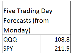
Here are forecasts of the weekly high price for three securities. These include intensely traded exchange traded funds (ETF’s) and a blue chip stock – QQQ, SPY, and GE.

TableA27

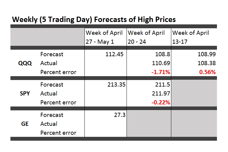
The table also shows the track record so far.

All the numbers not explicitly indicated as percents are in US dollars.

These forecasts come with disclaimers. They are presented purely for scientific and informational purposes. This blog takes no responsibility for any investment gains or losses that might be linked with these forecasts. Invest at your own risk.

So having said that, some implications and background information.

First of all, it looks like it’s off to the races for the market as a whole this week, although possibly not for GE. The highs for the ETF’s all show solid gains.

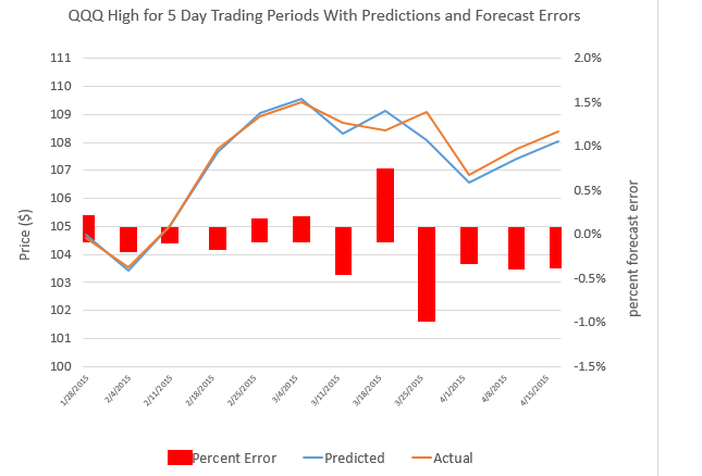
Note, too, that these are forecasts of the high price which will be reached over the next five trading days, Monday through Friday of this week.

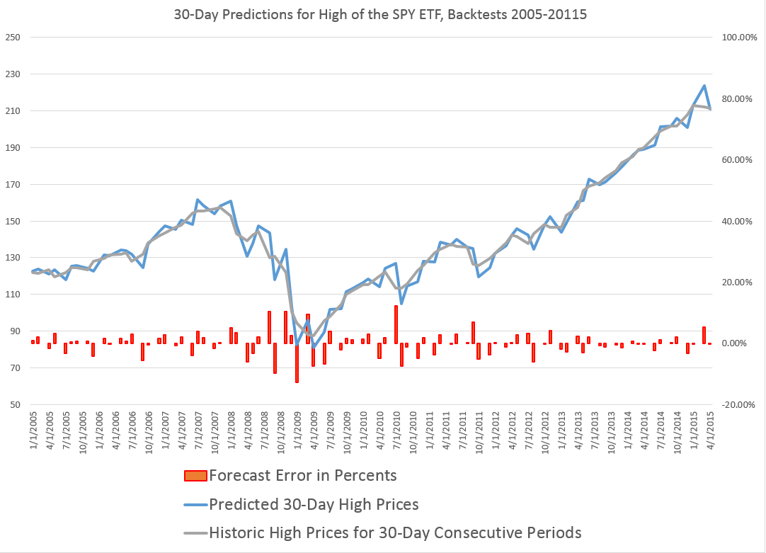
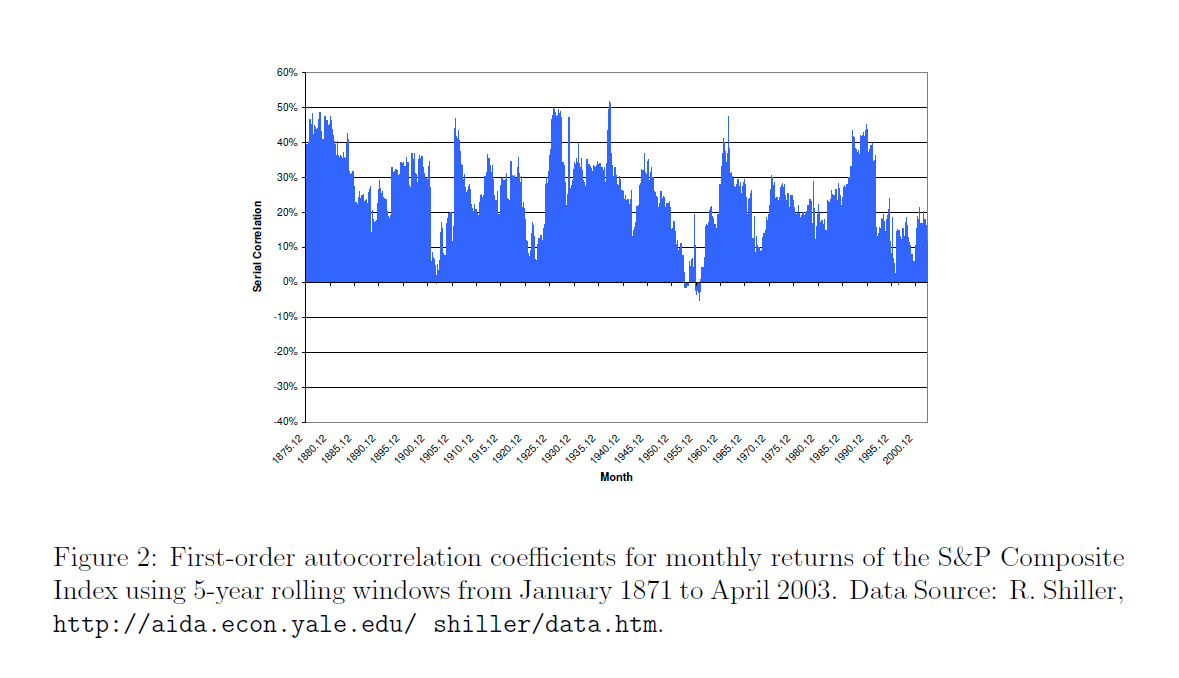
Key features of the method are now available in a white paper published under the auspices of the University of Munich – Predictability of the daily high and low of the S&P 500 index. This research shows that the so-called proximity variables achieve higher accuracies in predicting the daily high and low prices for the S&P 500 than do benchmark approaches, such as the no-change forecast and forecasts from an autoregressive model.

Again, caution is advised in making direct application of the methods in the white paper to the current problem –forecasting the high for a five day trading period. There have been many modifications.

That’s, of course, one reason for the public announcements of forecasts from the NPV (new proximity variable) model.

Go real-time, I’ve been advised. It makes the best case, or at least exposes the results to the light of day.

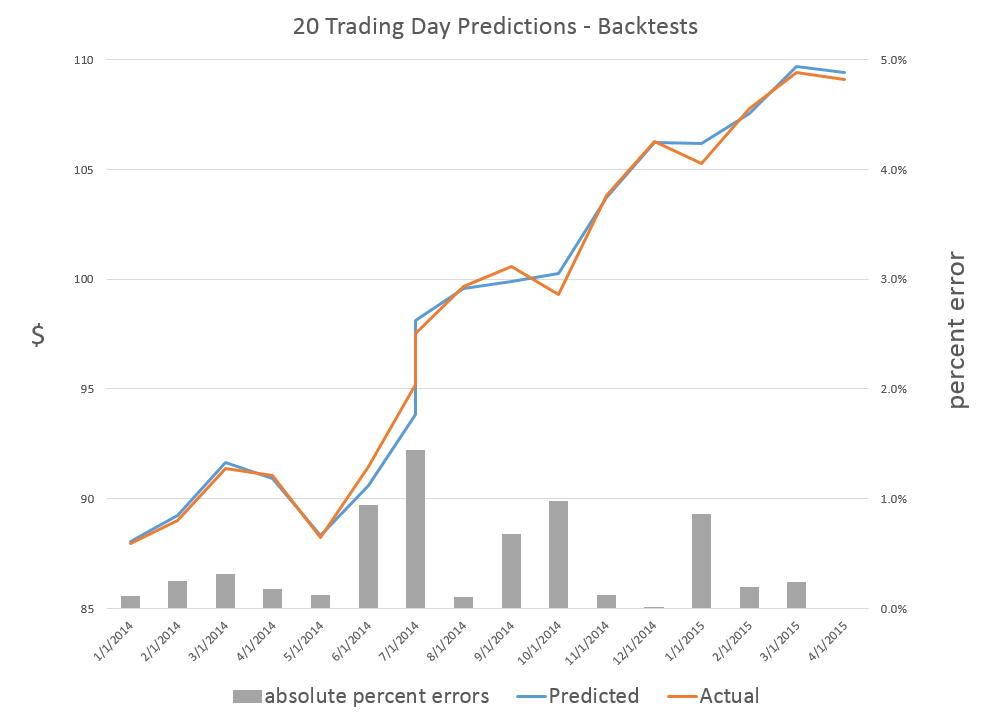
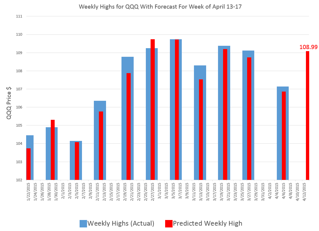
Based on backtesting, I expect forecasts for GE to be less accurate than those for QQQ and SPY. In terms of mean absolute percent error (MAPE), we are talking around 1% for QQQ and SPY and, maybe, 1.7% for GE.

The most reliable element of these forecasts are the indicated directions of change from the previous period highs.

Features and Implications

There are other several other features which are reliably predicted by the NPV models. For example, forecasts for the low price or even closing prices on Friday can be added – although closing prices are less reliable. Obviously, too, volatility metrics are implied by predictions of the high and low prices.

These five-trading day forecasts parallel the results for daily periods documented in the above-cited white paper. That is, the NPV forecast accuracy for these securities in each case beats “no-change” and autoregressive model forecasts.

Focusing on stock market forecasts has “kept me out of trouble” recently. I’m focused on quantitative modeling, and am not paying a lot of attention to global developments – such as the ever- impending Greek default or, possibly, exit from the euro. Other juicy topics include signs of slowing in the global economy, and the impact of armed conflict on the Arabian Peninsula on the global price of oil. These are great topics, but beyond hearsay or personal critique, it is hard to pin things down just now.

So, indeed, I may miss some huge external event which tips this frothy stock market into reverse – but, at the same time, I assure you, once a turning point from some external disaster takes place, the NPV models should do a good job of predicting the extent and duration of such a decline.

On a more optimistic note, my research shows the horizons for which the NPV approach applies and does a better job than the benchmark models. I have, for example, produced backtests for quarterly SPY data, demonstrating continuing superiority of the NPV method.

My guess – and I would be interested in validating this – is that the NPV approach connects with dominant trader practice. Maybe stock market prices are, in some sense, a random walk. But the reactions of traders to daily price movements create short term order out of randomness. And this order can emerge and persist for relatively long periods. And, not only that, but the NPV approach is linked with self-reinforcing tendencies, so that awareness may just make predicted effects more pronounced. That is, if I tell you the high price of a security is going up over the coming period, your natural reaction is to buy in – thus reinforcing the prediction. And the prediction is not just public relations stunt or fluff. The first prediction is algorithmic, rather than wishful and manipulative. Thus, the direction of change is more predictable than the precise extent of price change.

In any case, we will see over coming weeks how well these models do.

Some Comments on Forecasting High and Low Stock Prices

I want to pay homage to Paul Erdős, the eccentric Hungarian-British-American-Israeli mathematician, whom I saw lecture a few years before his death. Erdős kept producing work in mathematics into his 70’s and 80’s – showing this is quite possible. Of course, he took amphetamines and slept on people’s couches while he was doing this work in combinatorics, number theory, and probability.

erdos

In any case, having invoked Erdős, let me offer comments on forecasting high and low stock prices – a topic which seems to be terra incognita, for the most part, to financial research.

First, let’s take a quick look at a chart showing the maximum prices reached by the exchange traded fund QQQ over a critical period during the last major financial crisis in 2008-2009.

MaxHighChart

The graph charts five series representing QQQ high prices over periods extending from 1 day to 40 days.

The first thing to notice is that the variability of these time series decreases as the period for the high increases.

This suggests that forecasting the 40 day high could be easier than forecasting the high price for, say, tomorrow.

While this may be true in some sense, I want to point out that my research is really concerned with a slightly different problem.

This is forecasting ahead by the interval for the maximum prices. So, rather than a one-day-ahead forecast of the 40 day high price (which would include 39 known possible high prices), I forecast the high price which will be reached over the next 40 days.

This problem is better represented by the following chart.

Sampled5Highs

This chart shows the high prices for QQQ over periods ranging from 1 to 40 days, sampled at what you might call “40 day frequencies.”

Now I am not quite going to 40 trading day ahead forecasts yet, but here are results for backtests of the algorithm which produces 20-trading-day-ahead predictions of the high for QQQ.

20Dayforecast

The blue lines shows the predictions for the QQQ high, and the orange line indicates the actual QQQ highs for these (non-overlapping) 20 trading day intervals. As you can see, the absolute percent errors – the grey bars – are almost all less than 1 percent error.

Random Walk

Now, these results are pretty good, and the question arises – what about the random walk hypothesis for stock prices?

Recall that a simple random walk can be expressed by the equation xt=xt-1 + εt where εt is conventionally assumed to be distributed according to N(0,σ) or, in other words, as a normal distribution with zero mean and constant variance σ.

An interesting question is whether the maximum prices for a stock whose prices follow a random walk also can be described, mathematically, as a random walk.

This is elementary, when we consider that any two observations in a time series of random walks can be connected together as xt+k = xt + ω where ω is distributed according to a Gaussian distribution but does not necessarily have a constant variance for different values of the spacing parameter k.

From this it follows that the methods producing these predictions or forecasts of the high of QQQ over periods of several trading days also are strong evidence against the underlying QQQ series being a random walk, even one with heteroskedastic errors.

That is, I believe the predictability demonstrated for these series are more than cointegration relationships.

Where This is Going

While demonstrating the above point could really rock the foundations of finance theory, I’m more interested, for the moment, in exploring the extent of what you can do with these methods.

Very soon I’m going to post on how these methods may provide signals as to turning points in stock market prices.

Stay tuned, and thanks for your comments and questions.

Erdős picture from Encyclopaedia Britannica

Update and Extension – Weekly Forecasts of QQQ and Other ETF’s

Well, the first official forecast rolled out for QQQ last week.

It did relatively well. Applying methods I have been developing for the past several months, I predicted the weekly high for QQQ last week at 108.98.

In fact, the high price for QQQ for the week was 108.38, reached Monday, April 13.

This means the forecast error in percent terms was 0.55%.

It’s possible to look more comprehensively at the likely forecast errors with my approach with backtesting.

Here is a chart showing backtests for the “proximity variable method” for the QQQ high price for five day trading periods since the beginning of 2015.

QQQupdate

The red bars are errors, and, from their axis on the right, you can see most of these are below 0.5%.

This is encouraging, and there are several adjustments which may improve forecasting performance beyond this level of accuracy I want to explore.

So here is the forecast of the high prices that will be reached by QQQ and SPY for the week of April 20-24.

ForecastTab1

As you can see, I’ve added SPY, an ETF tracking the S&P500.

I put this up on Businessforecastblog because I seek to make a point – namely, that I believe methods I have developed can produce much more accurate forecasts of stock prices.

It’s often easier and more compelling to apply forecasting methods and show results, than it is to prove theoretically or otherwise argue that a forecasting method is worth its salt.

Disclaimer –  These forecasts are for informational purposes only. If you make investments based on these numbers, it is strictly your responsibility. Businessforecastblog is not responsible or liable for any potential losses investors may experience in their use of any forecasts presented in this blog.

Well, I am working on several stock forecasts to add to projections for these ETF’s – so will expand this feature in forthcoming Mondays.

Predicting the High Reached by the SPY ETF 30 Days in Advance – Some Results

Here are some backtests of my new stock market forecasting procedures.

Here, for example, is a chart showing the performance of what I call the “proximity variable approach” in predicting the high price of the exchange traded fund SPY over 30 day forward periods (click to enlarge).

3oDaySPY

So let’s be clear what the chart shows.

The proximity variable approach- which so far I have been abbreviating as “PVar” – is able to identify the high prices reached by the SPY in the coming 30 trading days with forecast errors mostly under 5 percent. In fact, the MAPE for this approximately ten year period is 3 percent. The percent errors, of course, are charted in red with their metric on the axis to the right.

The blue line traces out the predictions, and the grey line shows the actual highs by 30 trading day period.

These results far surpass what can be produced by benchmark models, such as the workhorse No Change model, or autoregressive models.

Why not just do this month-by-month?

Well, months have varying numbers of trading days, and I have found I can boost accuracy by stabilizing the number of trading days considered in the algorithm.

Comments

Realize, of course, that a prediction of the high price that a stock or ETF will reach in a coming period does not tell you when the high will be reached – so it does not immediately translate to trading profits. The high in question could come with the opening price of the period, for example, leaving you out of the money, if you hear there is this big positive prediction of growth and then jump in the market.

However, I do think that market participants react to anticipated increases or decreases in the high or low of a security.

You might explain these results as follows. Traders react to fairly simple metrics predicting the high price which will be reached in the next period – and let this concept be extensible from a day to a month in this discussion. In so reacting, these traders tend to make such predictive models self-fulfilling.

Therefore, daily prices – the opening, the high, the low, and the closing prices – encode a lot more information about trader responses than is commonly given in the literature on stock market forecasting.

Of course, increasingly, scholars and experts are chipping away at the “efficient market hypothesis” and showing various ways in which stock market prices are predictable, or embody an element of predictability.

However, combing Google Scholar and other sources, it seems almost no one has taken the path to modeling stock market prices I am developing here. The focus in the literature is on closing prices and daily returns, for example, rather than high and low prices.

I can envision a whole research program organized around this proximity variable approach, and am drawn to taking this on, reporting various results on this blog.

If any readers would like to join with me in this endeavor, or if you know of resources which would be available to support such a project – feel free to contact me via the Comments and indicate, if you wish, whether you want your communication to be private.

Let’s Get Real Here – QQQ Stock Price Forecast for Week of April 13-17

The thing I like about forecasting is that it is operational, rather than merely theoretical. Of course, you are always wrong, but the issue is “how wrong?” How close do the forecasts come to the actuals?

I have been toiling away developing methods to forecast stock market prices. Through an accident of fortune, I have come on an approach which predicts stock prices more accurately than thought possible.

After spending hundreds of hours over several months, I am ready to move beyond “backtesting” to provide forward-looking forecasts of key stocks, stock indexes, and exchange traded funds.

For starters, I’ve been looking at QQQ, the PowerShares QQQ Trust, Series 1.

Invesco describes this exchange traded fund (ETF) as follows:

PowerShares QQQ™, formerly known as “QQQ” or the “NASDAQ- 100 Index Tracking Stock®”, is an exchange-traded fund based on the Nasdaq-100 Index®. The Fund will, under most circumstances, consist of all of stocks in the Index. The Index includes 100 of the largest domestic and international nonfinancial companies listed on the Nasdaq Stock Market based on market capitalization. The Fund and the Index are rebalanced quarterly and reconstituted annually.

This means, of course, that QQQ has been tracking some of the most dynamic elements of the US economy, since its inception in 1999.

In any case, here is my forecast, along with tracking information on the performance of my model since late January of this year.

QQQForecast

The time of this blog post is the morning of April 13, 2015.

My algorithms indicate that the high for QQQ this week will be around $109 or, more precisely, $108.99.

So this is, in essence, a five day forecast, since this high price can occur in any of the trading days of this week.

The chart above shows backtests for the algorithm for ten weeks. The forecast errors are all less than 0.65% over this history with a mean absolute percent error (MAPE) of 0.34%.

So that’s what I have today, and count on succeeding installments looking back and forward at the beginning of the next several weeks (Monday), insofar as my travel schedule allows this.

Also, my initial comments on this post appear to offer a dig against theory, but that would be unfair, really, since “theory” – at least the theory of new forecasting techniques and procedures – has been very important in my developing these algorithms. I have looked at residuals more or less as a gold miner examines the chat in his pan. I have considered issues related to the underlying distribution of stock prices and stock returns – NOTE TO THE UNINITIATED – STOCK PRICES ARE NOT NORMALLY DISTRIBUTED. There is indeed almost nothing about stocks or stock returns which is related to the normal probability distribution, and I think this has been a huge failing of conventional finance, the Black Scholes Theorem, and the like.

So theory is important. But you can’t stop there.

This should be interesting. Stay tuned. I will add other securities in coming weeks, and provide updates of QQQ forecasts.

Readers interested in the underlying methods can track back on previous blog posts (for example, Pvar Models for Forecasting Stock Prices or Time-Varying Coefficients and the Risk Environment for Investing).

Stock Trading – Volume and Volatility

What about the relationship between the volume of trades and stock prices? And while we are on the topic, how about linkages between volume, volatility, and stock prices?

These questions have absorbed researchers for decades, recently drawing forth very sophisticated analysis based on intraday data.

I highlight big picture and key findings, and, of course, cannot resolve everything. My concern is not to be blindsided by obvious facts.

Relation Between Stock Transactions and Volatility

One thing is clear.

From a “macrofinancial” perspective, stock volumes, as measured by transactions, and volatility, as measured by the VIX volatility index, are essentially the same thing.

This is highlighted in the following chart, based on NYSE transactions data obtained from the Facts and Figures resource maintained by the Exchange Group.

VIXandNYSETrans

Now eyeballing this chart, it is possible, given this is daily data, that there could be slight lags or leads between these variables. However, the greatest correlation between these series is contemporaneous. Daily transactions and the closing value of the VIX move together trading day by trading day.

And just to bookmark what the VIX is, it is maintained by the Chicago Board Options Exchange (CBOE) and

The CBOE Volatility Index® (VIX®) is a key measure of market expectations of near-term volatility conveyed by S&P 500 stock index option prices. Since its introduction in 1993, VIX has been considered by many to be the world’s premier barometer of investor sentiment and market volatility. Several investors expressed interest in trading instruments related to the market’s expectation of future volatility, and so VIX futures were introduced in 2004, and VIX options were introduced in 2006.

Although the CBOE develops the VIX via options information, volatility in conventional terms is a price-based measure, being variously calculated with absolute or squared returns on closing prices.

Relation Between Stock Prices and Volume of Transactions

As you might expect, the relation between stock prices and the volume of stock transactions is controversial

It seems reasonable there should be a positive relationship between changes in transactions and price changes. However, shifts to the downside can trigger or be associated with surges in selling and higher volume. So, at the minimum, the relationship probably is asymmetric and conditional on other factors.

The NYSE data in the graph above – and discussed more extensively in the previous post – is valuable, when it comes to testing generalizations.

Here is a chart showing the rate of change in the volume of daily transactions sorted or ranked by the rate of change in the average prices of stocks sold each day on the New York Stock Exchange (click to enlarge).

delPdelT

So, in other words, array the daily transactions and the daily average price of stocks sold side-by-side. Then, calculate the day-over-day growth (which can be negative of course) or rate of change in these variables. Finally, sort the two columns of data, based on the size and sign of the rate of change of prices – indicated by the blue line in the above chart.

This chart indicates the largest negative rates of daily change in NYSE average prices are associated with the largest positive changes in daily transactions, although the data is noisy. The trendline for the rate of transactions data is indicated by the trend line in red dots.

The relationship, furthermore, is slightly nonlinear,and weak.

There may be more frequent or intense surges to unusual levels in transactions associated with the positive side of the price change chart. But, if you remove “outliers” by some criteria, you colud find that the average level of transactions tends to be higher for price drops, that for price increases, except perhaps for the highest price increases.

As you might expect from the similarity of the stock transactions volume and VIX series, a similar graph can be cooked up showing the rates of change for the VIX, ranked by rates of change in daily average prices of stock on the NYSE.

delPdelVIX

Here the trendline more clearly delineates a negative relationship between rates of change in the VIX and rates of change of prices – as, indeed, the CBOE site suggests, at one point.

Its interesting a high profile feature of the NYSE and, presumably, other exchanges – volume of stock transactions – has, by some measures, only a tentative relationship with price change.

I’d recommend several articles on this topic:

The relation between price changes and trading volume: a survey (from the 1980’s, no less)

Causality between Returns and Traded Volumes (from the late 1990’)

The bivariate GARCH approach to investigating the relation between stock returns, trading volume, and return volatility (from 2011)

The plan is to move on to predictability issues for stock prices and other relevant market variables in coming posts.

Trading Volume- Trends, Forecasts, Predictive Role

The New York Stock Exchange (NYSE) maintains a data library with historic numbers on trading volumes. Three charts built with some of this data tell an intriguing story about trends and predictability of volumes of transactions and dollars on the NYSE.

First, the number of daily transactions peaked during the financial troubles of 2008, only showing some resurgence lately.

transvol

This falloff in the number of transactions is paralleled by the volume of dollars spent in these transactions.

dollartrans

These charts are instructive, since both highlight the existence of “spikes” in transaction and dollar volume that would seem to defy almost any run-of-the-mill forecasting algorithm. This is especially true for the transactions time series, since the spikes are more irregularly spaced. The dollar volume time series suggests some type of periodicity is possible for these spikes, particularly in recent years.

But lower trading volume has not impacted stock prices, which, as everyone knows, surged past 2008 levels some time ago.

A raw ratio between the value of trades and NYSE stock transactions gives the average daily price per transaction.

vluepershare

So stock prices have rebounded, for the most part, to 2008 levels. Note here that the S&P 500 index stocks have done much better than this average for all stocks.

Why has trading volume declined on the NYSE? Some reasons gleaned from the commentariat.

  1. Mom and Pop traders largely exited the market, after the crash of 2008
  2. Some claim that program trading or high frequency trading peaked a few years back, and is currently in something of a decline in terms of its proportion of total stock transactions. This is, however, not confirmed by the NYSE Facts and Figures, which shows program trading pretty consistently at around 30 percent of total trading transactions..
  3. Interest has shifted to options and futures, where trading volumes are rising.
  4. Exchange Traded Funds (ETF’s) make up a larger portion of the market, and they, of course, do not actively trade.
  5. Banks have reduced their speculation in equities, in anticipation of Federal regulations

See especially Market Watch and Barry Ritholtz on these trends.

But what about the impact of trading volume on price? That’s the real zinger of a question I hope to address in coming posts this week.

Time-Varying Coefficients and the Risk Environment for Investing

My research provides strong support for variation of key forecasting parameters over time, probably reflecting the underlying risk environment facing investors. This type of variation is suggested by Lo ( 2005).

So I find evidence for time varying coefficients for “proximity variables” that predict the high or low of a stock in a period, based on the spread between the opening price and the high or low price of the previous period.

Figure 1 charts the coefficients associated with explanatory variables that I call OPHt and OPLt. These coefficients are estimated in rolling regressions estimated with five years of history on trading day data for the S&P 500 stock index. The chart is generated with more than 3000 separate regressions.

Here OPHt is the difference between the opening price and the high of the previous period, scaled by the high of the previous period. Similarly, OPLt is the difference between the opening price and the low of the previous period, scaled by the low of the previous period. Such rolling regressions sometimes are called “adaptive regressions.”

Figure 1 Evidence for Time Varying Coefficients – Estimated Coefficients of OPHt and OPLt Over Study Sample

TvaryCoeff

Note the abrupt changes in the values of the coefficients of OPHt and OPLt in 2008.

These plausibly reflect stock market volatility in the Great Recession. After 2010 the value of both coefficients tends to move back to levels seen at the beginning of the study period.

This suggests trajectories influenced by the general climate of risk for investors and their risk preferences.

I am increasingly convinced the influence of these so-called proximity variables is based on heuristics such as “buy when the opening price is greater than the previous period high” or “sell, if the opening price is lower than the previous period low.”

Recall, for example, that the coefficient of OPHt measures the influence of the spread between the opening price and the previous period high on the growth in the daily high price.

The trajectory, shown in the narrow, black line, trends up in the approach to 2007. This may reflect investors’ greater inclination to buy the underlying stocks, when the opening price is above the previous period high. But then the market experiences the crisis of 2008, and investors abruptly back off from their eagerness to respond to this “buy” signal. With onset of the Great Recession, investors become increasingly risk adverse to such “buy” signals, only starting to recover their nerve after 2013.

A parallel interpretation of the trajectory of the coefficient of OPLt can be developed based on developments 2008-2009.

Time variation of these coefficients also has implications for out-of-sample forecast errors.

Thus, late 2008, when values of the coefficients of both OPH and OPL make almost vertical movements in opposite directions, is the period of maximum out-of-sample forecast errors. Forecast errors for daily highs, for example, reach a maximum of 8 percent in October 2008. This can be compared with typical errors of less than 0.4 percent for out-of-sample forecasts of daily highs with the proximity variable regressions.

Heuristics

Finally, I recall a German forecasting expert discussing heuristics with an example from baseball. I will try to find his name and give him proper credit. By the idea is that an outfielder trying to catch a flyball does not run calculations involving mass, angle, velocity, acceleration, windspeed, and so forth. Instead, basically, an outfielder runs toward the flyball, keeping it at a constant angle in his vision, so that it falls then into his glove at the last second. If the ball starts descending in his vision, as he approaches it, it may fall on the ground before him. If it starts to float higher in his perspective as he runs to get under it, it may soar over him, landing further back int he field.

I wonder whether similar arguments can be advanced for the strategy of buying based or selling based on spreads between the opening price in a period and the high and low prices in a previous period.

How Did My Forecast of the SPY High and Low Issued January 22 Do?

A couple of months ago, I applied the stock market forecasting approach based on what I call “proximity variables” to forward-looking forecasts – as opposed to “backcasts” testing against history.

I’m surprised now that I look back at this, because I offered a forecast for 40 trading days (a little foolhardy?).

In any case, I offered forecasts for the high and low of the exchange traded fund SPY, as follows:

What about the coming period of 40 trading days, starting from this morning’s (January 22, 2015) opening price for the SPY – $203.99?

Well, subject to qualifications I will state further on here, my estimates suggest the high for the period will be in the range of $215 and the period low will be around $194. Cents attached to these forecasts would be, of course, largely spurious precision.

In my opinion, these predictions are solid enough to suggest that no stock market crash is in the cards over the next 40 trading days, nor will there be a huge correction. Things look to trade within a range not too distant from the current situation, with some likelihood of higher highs.

It sounds a little like weather forecasting.

Well, 27 trading days have transpired since January 22, 2015 – more than half the proposed 40 associated with the forecast.

How did I do?

Here is a screenshot of the Yahoo Finance table showing opening, high, low, and closing prices since January 22, 2015.

SPYJan22etpassim

The bottom line – so far, so good. Neither the high nor low of any trading day has broached my proposed forecasts of $194 for the low and $215 for the high.

Now, I am pleased – a win just out of the gates with the new modeling approach.

However, I would caution readers seeking to use this for investment purposes. This approach recommends shorter term forecasts to focus in on the remaining days of the original forecast period. So, while I am encouraged the $215 high has not been broached, despite the hoopla about recent gains in the market, I don’t recommend taking $215 as an actual forecast at this point for the remaining 13 trading days – two or three weeks. Better forecasts are available from the model now.

“What are they?”

Well, there are a lot of moving parts in the computer programs to make these types of updates.

Still, it is interesting and relevant to forecasting practice – just how well do the models perform in real time?

So I am planning a new feature, a periodic update of stock market forecasts, with a look at how well these did. Give me a few days to get this up and running.

More on the “Efficiency” of US Stock Markets – Evidence from 1871 to 2003

In a pivotal article, Andrew Lo writes,

Many of the examples that behavioralists cite as violations of rationality that are inconsistent with market efficiency loss aversion, overconfidence, overreaction, mental accounting, and other behavioral biases are, in fact, consistent with an evolutionary model of individuals adapting to a changing environment via simple heuristics.

He also supplies an intriguing graph of the rolling first order autocorrelation of monthly returns of the S&P Composite Index from January 1971 to April 2003.

LoACchart

Lo notes the Random Walk Hypothesis implies that returns are serially uncorrelated, so the serial correlation coefficient ought to be zero – or at least, converging to zero over time as markets move into equilibrium.

However, the above chart shows this does not happen, although there are points in time when the first order serial correlation coefficient is small in magnitude, or even zero.

My point is that the first order serial correlation in daily returns for the S&P 500 is large enough for long enough periods to generate profits above a Buy-and-Hold strategy – that is, if one can negotiate the tricky milliseconds of trading at the end of each trading day.