Sales Forecasts and Incentives

In some contexts, the problem is to find out what someone else thinks the best forecast is.

Thus, management may want to have accurate reporting or forecasts from the field sales force of “sales in the funnel” for the next quarter.

In a widely reprinted article from the Harvard Business Review, Gonik shows how to design sales bonuses to elicit the best estimates of future sales from the field sales force. The publication dates from the 1970’s, but is still worth considering, and has become enshrined in the management science literature.

Quotas are set by management, and forecasts or sales estimates are provided by the field salesforce.

In Gonik’s scheme, salesforce bonus percentages are influenced by three factors: actual sales volume, sales quota, and the forecast of sales provided from the field.

Consider the following bonus percentages (click to enlarge).

 Gonik                      

Grid coordinates across the top are the sales agent’s forecast divided by the quota.

Actual sales divided by the sales quota are listed down the left column of the table.

Suppose the quota from management for a field sales office is $50 million in sales for a quarter. This is management’s perspective on what is possible, given first class effort.

The field sales office, in turn, has information on the scope of repeat and new customer sales that are likely in the coming quarter. The sales office forecasts, conservatively, that they can sell $25 million in the next quarter.

This situates the sales group along the column under a Forecast/Quota figure of 0.5.

Then, it turns out that, lo and behold, the field sales office brings in $50 million in sales by the end of the quarter in question.

Their bonus, accordingly, is determined by the row labeled “100″ – for 100% of sales to quota. Thus, the field sales office gets a bonus which is 90 percent of the standard bonus for that period, whatever that is.

Naturally, the salesmen will see that they left money on the table. If they had forecast $50 million in sales for the quarter and achieved it, they would have 120 percent of the standard quota.

Notice that the diagonal highlighted in green shows the maximum bonus percentages for any given ratio of actual sales to quota (any given row). These maximum bonus percents are exactly at the intersection where the ratio of actual sales to quota equals the ratio of sales forecast to quota.

The area of the table colored in pink identifies a situation in which the sales forecasts exceed the actual sales.

The portion of the table highlighted in light blue, on the other hand, shows the cases in which the actual sales exceed the forecast.

This bonus setup provides monetary incentives for the sales force to accurately report their best estimates of prospects in the field, rather than “lowballing” the numbers. And just to review the background to the problem – management sometimes considers that the sales force is likely to under-report opportunities, so they look better when these are realized.

This setup has been applied by various companies, including IBM, and is enshrined in the management literature.

The algebra to develop a table of percentages like the one shown is provided in an article by Mantrala and Rama.

These authors also point out a similarity between Gonik’s setup and reforms of central planning in the old Soviet Union and communist Hungary. This odd association should not discredit the Gonik scheme in anyone’s mind. Instead, the linkage really highlights how fundamental the logic of the bonuses table is. In my opinion, Soviet Russia experienced economic collapse for entirely separate reasons – primarily failures of the pricing system and reluctance to permit private ownership of assets.

A subsequent post will consider business-to-business (B2B) supply contracts and related options frameworks which provide incentives for sharing demand or forecast information along the supply chain.

Predicting the Stock Market, Making Profits in the Stock Market

Often, working with software and electronics engineers, a question comes up – “if you are so good at forecasting (company sales, new product introductions), why don’t you forecast the stock market?” This might seem to be a variant of “if you are so smart, why aren’t you rich?” but I think it usually is asked more out of curiosity, than malice.

In any case, my standard reply has been that basically you could not forecast the stock market; that the stock market was probably more or less a random walk. If it were possible to forecast the stock market, someone would have done it. And the effect of successful forecasts would be to nullify further possibility of forecasting. I own an early edition of Burton Malkiel’s Random Walk Down Wall Street.

Today, I am in the amazing position of earnestly attempting to bring attention to the fact that, at least since 2008, a major measure of the stock market – the SPY ETF which tracks the S&P 500 Index, in fact, can be forecast. Or, more precisely, a forecasting model for daily returns of the SPY can lead to sustainable, increasing returns over the past several years, despite the fact the forecasting model, is, by many criteria, a weak predictor.

I think this has to do with special features of this stock market time series which have not, heretofore, received much attention in econometric modeling.

So here are the returns from applying this SPY from early 2008 to early 2014 (click to enlarge).

SPYTradingProgramcompBH

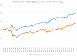
I begin with a $1000 investment 1/22/2008 and trade potentially every day, based on either the Trading Program or a Buy & Hold strategy.

Now there are several remarkable things about this Trading Program and the underlying regression model.

First, the regression model is a most unlikely candidate for making money in the stock market. The R2 or coefficient of determination is 0.0238, implying that the 60 regressors predict only 2.38 percent of the variation in the SPY rates of return. And it’s possible to go on in this vein – for example, the F-statistic indicating whether there is a relation between the regressors and the dependent variable is 1.42, just marginally above the 1 percent significance level, according to my reading of the Tables.

And the regression with 60 regressors correctly predicts the correct sign of the next days’ SPY rates of return only 50.1 percent of the time.

This, of course, is a key fact, since the Trading Program (see below) is triggered by positive predictions of the next day’s rate of return. When the next day rate of return is predicted to be positive and above a certain minimum value, the Trading Program buys SPY with the money on hand from previous sales – or, if the investor is already holding SPY because the previous day’s prediction also was positive, the investor stands pat.

The Conventional Wisdom

Professor Jim Hamilton, one of the principals (with Menzie Chin) in Econbrowser had a post recently On R-squared and economic prediction which makes the sensible point that R2 or the coefficient of determination in a regression is not a great guide to predictive performance. The post shows, among other things, that first differences of the daily S&P 500 index values regressed against lagged values of these first differences have low R2 – almost zero.

Hamilton writes,

Actually, there’s a well-known theory of stock prices that claims that an R-squared near zero is exactly what you should find. Specifically, the claim is that everything anybody could have known last month should already have been reflected in the value of pt -1. If you knew last month, when pt-1 was 1800, that this month it was headed to 1900, you should have bought last month. But if enough savvy investors tried to do that, their buy orders would have driven pt-1 up closer to 1900. The stock price should respond the instant somebody gets the news, not wait around a month before changing.

That’s not a bad empirical description of stock prices– nobody can really predict them. If you want a little fancier model, modern finance theory is characterized by the more general view that the product of today’s stock return with some other characteristics of today’s economy (referred to as the “pricing kernel”) should have been impossible to predict based on anything you could have known last month. In this formulation, the theory is confirmed– our understanding of what’s going on is exactly correct– only if when regressing that product on anything known at t – 1 we always obtain an R-squared near zero.

Well, I’m in the position here of seeking to correct one of my intellectual mentors. Although Professor Hamilton and I have never met nor communicated directly, I did work my way through Hamilton’s seminal book on time series analysis – and was duly impressed.

I am coming to the opinion that the success of this fairly low-power regression model on the SPY must have to do with special characteristics of the underlying distribution of rates of return.

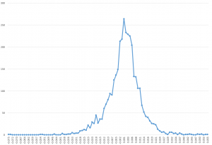
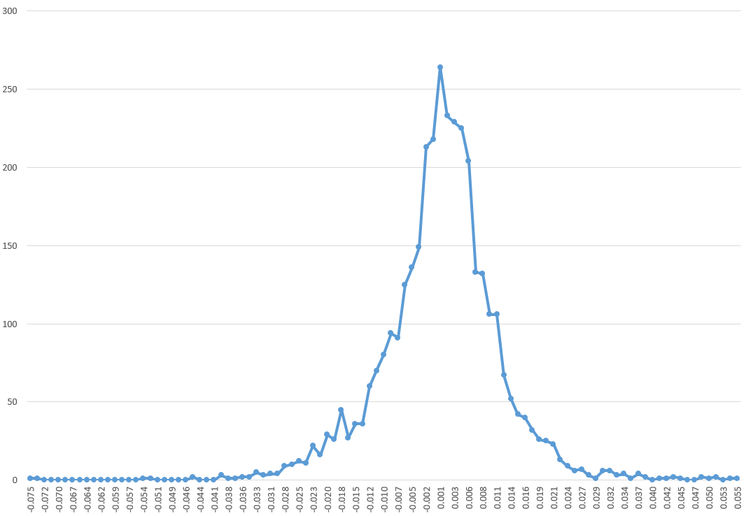
For example, it’s interesting that the correlations between the (61) regressors and the daily returns are higher, when the absolute values of the dependent variable rates of return are greater. There is, in fact, a lot of meaningless buzz at very low positive and negative rates of return. This seems consistent with the odd shape of the residuals of the regression, shown below.

RegResidualsSPY

I’ve made this point before, most recently in a post-2014 post Predicting the S&P 500 or the SPY Exchange-Traded Fund, where I actually provide coefficients for a autoregressive model estimated by Matlab’s arima procedure. That estimation, incidentally, takes more account of the non-normal characteristics of the distribution of the rates of return, employing a t-distribution in maximum likelihood estimates of the parameters. It also only uses lagged values of SPY daily returns, and does not include any contribution from the VIX.

I guess in the remote possibility Jim Hamilton glances at either of these posts, it might seem comparable to reading claims of a perpetual motion machine, a method to square the circle, or something similar- quackery or wrong-headedness and error.

A colleague with a Harvard Ph.D in applied math, incidentally, has taken the trouble to go over my data and numbers, checking and verifying I am computing what I say I am computing.

Further details follow on this simple ordinary least squares (OLS) regression model I am presenting here.

Data and the Model

The focus of this modeling effort is on the daily returns of the SPDR S&P 500 (SPY), calculated with daily closing prices, as -1+(today’s closing price/the previous trading day’s closing price). The data matrix includes 30 lagged values of the daily returns of the SPY (SPYRR) along with 30 lagged values of the daily returns of the VIX volatility index (VIXRR). The data span from 11/26/1993 to 1/16/2014 – a total of 5,072 daily returns.

There is enough data to create separate training and test samples, which is good, since in-sample performance can be a very poor guide to out-of-sample predictive capabilities. The training sample extends from 11/26/1993 to 1/18/2008, for a total of 3563 observations. The test sample is the complement of this, extending from 1/22/2008 to 1/16/2014, including 1509 cases.

So the basic equation I estimate is of the form

SPYRRt=a0+a1SPYRRt-1…a30SPYRRt-30+b1VIXRRt-1+..+b30VIXRRt-30

Thus, the equation has 61 parameters – 60 coefficients multiplying into the lagged returns for the SPY and VIX indices and a constant term.

Estimation Technique

To make this simple, I estimate the above equation with the above data by ordinary least squares, implementing the standard matrix equation b = (XTX)-1XTY, where T indicates ‘transpose.’ I add a leading column of ‘1’s’ to the data matrix X to allow for a constant term a0. I do not mean center or standardize the observations on daily rates of return.

Rule for Trading Program and Summing UP

The Trading Program is the same one I described in earlier blog posts on this topic. Basically, I update forecasts every day and react to the forecast of the next day’s daily return. If it is positive, and now above a certain minimum, I either buy or hold. If it is not, I sell or do not enter the market. Oh yeah, I start out with $1000 in all these simulations and only trade with proceeds from this initial investment.

The only element of unrealism is that I have to predict the closing price of the SPY some short period before the close of the market to be able to enter my trade. I have not looked closely at this, but I am assuming volatility in the last few seconds is bounded, except perhaps in very unusual circumstances.

I take the trouble to present the results of an OLS regression to highlight the fact that what looks like a weak model in this context can work to achieve profits. I don’t think that point has ever been made. There are, of course, all sorts of possibilities for further optimizing this model.

I also suspect that monetary policy has some role in the success of this Trading Program over this period – so it would be interesting to look at similar models at other times and perhaps in other markets.

Links – February 1, 2014

IT and Big Data

Kayak and Big Data Kayak is adding prediction of prices of flights over the coming 7 days to its meta search engine for the travel industry.

China’s Lenovo steps into ring against Samsung with Motorola deal Lenovo Group, the Chinese technology company that earns about 80 percent of its revenue from personal computers, is betting it can also be a challenger to Samsung Electronics Co Ltd and Apple Inc in the smartphone market.

5 Things To Know About Cognitive Systems and IBM Watson Rob High video on Watson at http://www.redbooks.ibm.com/redbooks.nsf/pages/watson?Open. Valuable to review. Watson is probably different than you think. Deep natural language processing.

Playing Computer Games and Winning with Artificial Intelligence (Deep Learning) Pesents the first deep learning model to successfully learn control policies directly from high-dimensional sensory input using reinforcement learning. The model is a convolutional neural network, trained with a variant of Q-learning, whose input is raw pixels and whose output is a value function estimating future rewards… [applies] method to seven Atari 2600 games from the Arcade Learning Environment, with no adjustment of the architecture or learning algorithm…outperforms all previous approaches on six of the games and surpasses a human expert on three of them.

Global Economy

China factory output points to Q1 lull Chinese manufacturing activity slipped to its lowest level in six months, with indications of slowing growth for the quarter to come in the world’s second-largest economy.

Japan inflation rises to a 5 year high, output rebounds Japan’s core consumer inflation rose at the fastest pace in more than five years in December and the job market improved, encouraging signs for the Bank of Japan as it seeks to vanquish deflation with aggressive money printing.

Coup Forecasts for 2014

coupforecast                       

World risks deflationary shock as BRICS puncture credit bubbles Ambrose Evans-Pritchard does some nice analysis in this piece.

Former IMF Chief Economist, Now India’s Central Bank Governor Rajan Takes Shot at Bernanke’s Destabilizing Policies

Some of his key points:

Emerging markets were hurt both by the easy money which flowed into their economies and made it easier to forget about the necessary reforms, the necessary fiscal actions that had to be taken, on top of the fact that emerging markets tried to support global growth by huge fiscal and monetary stimulus across the emerging markets. This easy money, which overlaid already strong fiscal stimulus from these countries. The reason emerging markets were unhappy with this easy money is “This is going to make it difficult for us to do the necessary adjustment.” And the industrial countries at this point said, “What do you want us to do, we have weak economies, we’ll do whatever we need to do. Let the money flow.”

Now when they are withdrawing that money, they are saying, “You complained when it went in. Why should you complain when it went out?” And we complain for the same reason when it goes out as when it goes in: it distorts our economies, and the money coming in made it more difficult for us to do the adjustment we need for the sustainable growth and to prepare for the money going out

International monetary cooperation has broken down. Industrial countries have to play a part in restoring that, and they can’t at this point wash their hands off and say we’ll do what we need to and you do the adjustment. ….Fortunately the IMF has stopped giving this as its mantra, but you hear from the industrial countries: We’ll do what we have to do, the markets will adjust and you can decide what you want to do…. We need better cooperation and unfortunately that’s not been forthcoming so far.

Science Perspective

Researchers Discover How Traders Act Like Herds And Cause Market Bubbles

Building on similarities between earthquakes and extreme financial events, we use a self-organized criticality-generating model to study herding and avalanche dynamics in financial markets. We consider a community of interacting investors, distributed in a small-world network, who bet on the bullish (increasing) or bearish (decreasing) behavior of the market which has been specified according to the S&P 500 historical time series. Remarkably, we find that the size of herding-related avalanches in the community can be strongly reduced by the presence of a relatively small percentage of traders, randomly distributed inside the network, who adopt a random investment strategy. Our findings suggest a promising strategy to limit the size of financial bubbles and crashes. We also obtain that the resulting wealth distribution of all traders corresponds to the well-known Pareto power law, while that of random traders is exponential. In other words, for technical traders, the risk of losses is much greater than the probability of gains compared to those of random traders. http://pre.aps.org/abstract/PRE/v88/i6/e062814

Blogs review: Getting rid of the Euler equation – the equation at the core of modern macro The Euler equation is one of the fundamentals, at a deep level, of dynamic stochastic general equilibrium (DSGE) models promoted as the latest and greatest in theoretical macroeconomics. After the general failures in mainstream macroeconomics with 2008-09, DGSE have come into question, and this review is interesting because it suggests, to my way of thinking, that the Euler equation linking past and future consumption patterns is essentially grafted onto empirical data artificially. It is profoundly in synch with neoclassical economic theory of consumer optimization, but cannot be said to be supported by the data in any robust sense. Interesting read with links to further exploration.

BOSTON COLLOQUIUM FOR PHILOSOPHY OF SCIENCE: Revisiting the Foundations of Statistics – check this out – we need the presentations online.