When time series data are available in frequencies higher than quarterly or monthly, many forecasting programs hit a wall in analyzing seasonal effects.
Researchers from the Australian Monash University published an interesting paper in the Journal of the American Statistical Association (JASA), along with an R program, to handle this situation – what can be called “complex seasonality.”
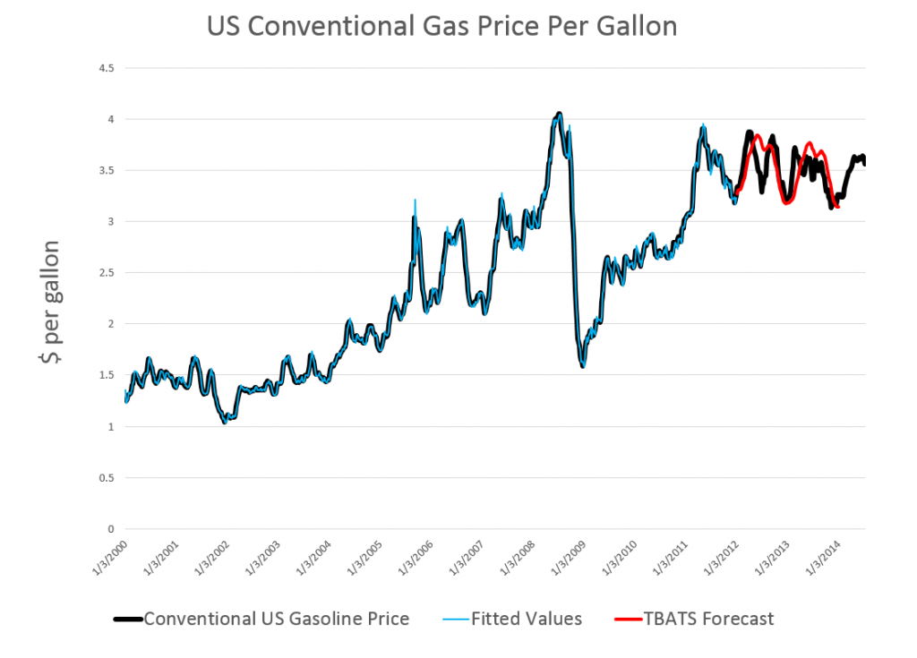
I’ve updated and modified one of their computations – using weekly, instead of daily, data on US conventional gasoline prices – and find the whole thing pretty intriguing.
If you look at the color codes in the legend below the chart, it’s a little easier to read and understand.
Here’s what I did.
I grabbed the conventional weekly US gasoline prices from FRED. These prices are for “regular” – the plain vanilla choice at the pump. I established a start date of the first week in 2000, after looking the earlier data over. Then, I used tbats(.) in the Hyndman R Forecast package which readers familiar with this site know can be downloaded for use in the open source matrix programming language R.
Then, I established an end date for a time series I call newGP of the first week in 2012, forecasting ahead with the results of applying tbats(.) to the historic data from 2000:1 to 2012:1 where the second number refers to weeks which run from 1 to 52. Note that some data scrubbing is needed to shoehorn the gas price data into 52 weeks on a consistent basis. I averaged “week 53” with the nearest acceptable week (either 52 or 1 in the next year), and then got rid of the week 53’s.
The forecast for 104 weeks is shown by the solid red line in the chart above.
This actually looks promising, as if it might encode some useful information for, say, US transportation agencies.
A draft of the JASA paper is available as a PDF download. It’s called Forecasting time series with complex seasonal patterns using exponential smoothing and in addition to daily US gas prices, analyzes daily electricity demand in Turkey and bank call center data.
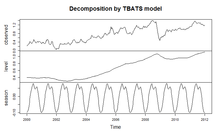
I’m only going part of the way to analyzing the gas price data, since I have not taken on daily data yet. But the seasonal pattern identified by tbats(.) from the weekly data is interesting and is shown below.
The weekly frequency may enable us to “get inside” a mid-year wobble in the pattern with some precision. Judging from the out-of-sample performance of the model, this “wobble” can in some cases be accentuated and be quite significant.
Trignometric series fit to the higher frequency data extract the seasonal patterns in tbats(.), which also features other advanced features, such as a capability for estimating ARMA (autoregressive moving average) models for the residuals.
I’m not fully optimizing the estimation, but these results are sufficiently strong to encourage exploring the toggles and switches on the routine.
Another routine which works at this level of aggregation is the stlf(.) routine. This is uses STL decomposition described in some detail in Chapter 36 Patterns Discovery Based on Time-Series Decomposition in a collection of essays on data mining.
Thoughts
Good forecasting software elicits sort of addictive behavior, when initial applications of routines seem promising. How much better can the out-of-sample forecasts be made with optimization of the features of the routine? How well does the routine do when you look at several past periods? There is even the possibility of extracting further information from the residuals through bootstrapping or bagging at some point. I think there is no other way than exhaustive exploration.
The payoff to the forecaster is the amazement of his or her managers, when features of a forecast turn out to be spot-on, prescient, or what have you – and this does happen with good software. An alternative, for example, to the Hyndman R Forecast package is the program STAMP I also am exploring. STAMP has been around for many years with a version running – get this – on DOS, which appears to have had more features than the current Windows incarnation. In any case, I remember getting a “gee whiz” reaction from the executive of a regional bus district once, relating to ridership forecasts. So it’s fun to wring every possible pattern from the data.


