If you learned your statistical technique more than ten years ago, consider it necessary to learn a whole bunch of new methods. Boosting is certainly one of these.
Let me pick a leading edge of this literature here – boosting time series predictions.
Results
Let’s go directly to the performance improvements.
In Boosting multi-step autoregressive forecasts, (Souhaib Ben Taieb and Rob J Hyndman, International Conference on Machine Learning (ICML) 2014) we find the following Table applying boosted time series forecasts to two forecasting competition datasets –
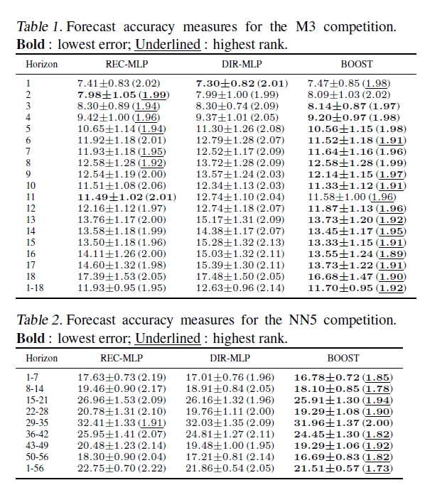
The three columns refer to three methods for generating forecasts over horizons of 1-18 periods (M3 Competition and 1-56 period (Neural Network Competition). The column labeled BOOST is, as its name suggests, the error metric for a boosted time series prediction. Either by the lowest symmetric mean absolute percentage error or a rank criterion, BOOST usually outperforms forecasts produced recursively from an autoregressive (AR) model, or forecasts from an AR model directly mapped onto the different forecast horizons.
There were a lot of empirical time series involved in these two datasets –
The M3 competition dataset consists of 3003 monthly, quarterly, and annual time series. The time series of the M3 competition have a variety of features. Some have a seasonal component, some possess a trend, and some are just fluctuating around some level. The length of the time series ranges between 14 and 126. We have considered time series with a range of lengths between T = 117 and T = 126. So, the number of considered time series turns out to be M = 339. For these time series, the competition required forecasts for the next H = 18 months, using the given historical data. The NN5 competition dataset comprises M = 111 time series representing roughly two years of daily cash withdrawals (T = 735 observations) at ATM machines at one of the various cities in the UK. For each time series, the competition required to forecast the values of the next H = 56 days (8 weeks), using the given historical data.
This research, notice of which can be downloaded from Rob Hyndman’s site, builds on the methodology of Ben Taieb and Hyndman’s recent paper in the International Journal of Forecasting A gradient boosting approach to the Kaggle load forecasting competition. Ben Taieb and Hyndman’s submission came in 5th out of 105 participating teams in this Kaggle electric load forecasting competition, and used boosting algorithms.
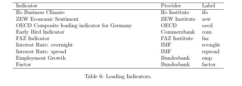
Let me mention a third application of boosting to time series, this one from Germany. So we have Robinzonov, Tutz, and Hothorn’s Boosting Techniques for Nonlinear Time Series Models (Technical Report Number 075, 2010 Department of Statistics University of Munich) which focuses on several synthetic time series and predictions of German industrial production.
Again, boosted time series models comes out well in comparisons.

GLMBoost or GAMBoost are quite competitive at these three forecast horizons for German industrial production.
What is Boosting?
My presentation here is a little “black box” in exposition, because boosting is, indeed, mathematically intricate, although it can be explained fairly easily at a very general level.
Weak predictors and weak learners play an important role in bagging and boosting –techniques which are only now making their way into forecasting and business analytics, although the machine learning community has been discussing them for more than two decades.
Machine learning must be a fascinating field. For example, analysts can formulate really general problems –
So we get the “definition” of boosting in general terms:
And a weak learner is a learning method that achieves only slightly better than chance correct classification of binary outcomes or labeling.
This sounds like the best thing since sliced bread.
But there’s more.
For example, boosting can be understood as a functional gradient descent algorithm.
Now I need to mention that some of the most spectacular achievements in boosting come in classification. A key text is the recent book Boosting: Foundations and Algorithms (Adaptive Computation and Machine Learning series) by Robert E. Schapire and Yoav Freund. This is a very readable book focusing on AdaBoost, one of the early methods and its extensions. The book can be read on Kindle and is starts out –
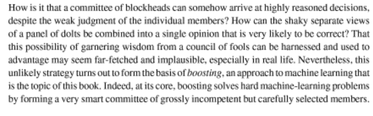
So worth the twenty bucks or so for the download.
The papers discussed above vis a vis boosting time series apply p-splines in an effort to estimate nonlinear effects in time series. This is really unfamiliar to most of us in the conventional econometrics and forecasting communities, so we have to start conceptualizing stuff like “knots” and component-wise fitting algortihms.
Fortunately, there is a canned package for doing a lot of the grunt work in R, called mboost.
Bottom line, I really don’t think time series analysis will ever be the same.