Category Archives: energy forecasting

Oil and Gas Prices II

One of the more interesting questions in applied forecasting is the relationship between oil and natural gas prices in the US market, shown below.

OIlGasPrices

Up to the early 1990’s, the interplay between oil and gas prices followed “rules of thumb” – for example, gas prices per million Btu were approximately one tenth oil prices.

There is still some suggestion of this – for example, peak oil prices recently hit nearly $140 a barrel, at the same time gas prices were nearly $14 per million Btu’s.

However, generally, ratio relationships appear to break down around 2009, if not earlier, during the first decade of the century.

A Longer Term Relationship?

Perhaps oil and gas prices are in a longer term relationship, but one disturbed in many cases in short run time periods.

One way economists and ecommetricians think of this is in terms of “co-integrating relationships.” That’s a fancy way of saying that regressions of the form,

Gas price in time t = constant + α(oil price in time t) + (residual in time t)

are predictive. Here, α is a coefficient to be estimated.

Now this looks like a straight-forward regression, so you might say – “what’s the problem?”

Well, the catch is that gas prices and oil prices might be nonstationary – that is, one or another form of a random walk.

If this is so – and positive results on standard tests such as the augmented Dickey Fuller (ADR) and Phillips-Peron are widely reported – there is a big potential problem. It’s easy to regress one completely unrelated nonstationary time series onto another, getting an apparently significant result, only to find this relationship disappears in the forecast. In other words two random series can, by chance, match up to each other over closely, but that’s no guarantee they will continue to do so.

Here’s where the concept of a co-integrating relationship comes into play.

If you can show, by various statistical tests, that variables are cointegrated, regressions such as the one above are more likely to be predictive.

Well, several econometric studies show gas and oil prices are in a cointegrated relationship, using data from the 1990’s through sometime in the first decade of the 2000’s. The more sophisticated specify auxiliary variables to account for weather or changes in gas storage. You might download and read, for example, a study published in 2007 under the auspices of the Dallas Federal Reserve Bank – What Drives Natural Gas Prices?

But it does not appear that this cointegrated relationship is fixed. Instead, it changes over time, perhaps exemplifying various regimes, i.e. periods of time in which the underlying parameters switch to new values, even though a determinate relationship can still be demonstrated.

Changing parameters are shown in the excellent 2012 study by Ramberg and Parsons in the Energy Journal – The Weak Tie Between Natural Gas and Oil Prices.

The Underlying Basis

Anyway, there are facts relating to production and use of oil and natural gas which encourage us to postulate a relationship in their prices, although the relationship may shift over time.

This makes sense since oil and gas are limited or completely substitutes in various industrial processes. This used to be more compelling in electric power generation, than it is today. According to the US Department of Energy, there are only limited amounts of electric power still produced by generators running on oil, although natural gas turbines have grown in importance.

Still, natural gas is often produced alongside of and is usually dissolved in oil, so oil and natural gas are usually joint products.

Recently, technology has changed the picture with respect to gas and oil.

On the demand side, the introduction of the combined-cycle combustion turbine made natural gas electricity generation more cost effective, thereby making natural gas in electric power generation even more dominant.

On the demand side, the new technologies of extracting shale oil and natural gas – often summarized under the rubric of “fracking” or hydraulic fracturing – have totally changed the equation, resulting in dramatic increases in natural gas supplies in the US.

This leaves the interesting question of what sort of forecasting model for natural gas might be appropriate.

Oil and Gas Prices – a “Golden Swan”?

Crude oil prices plummeted last week, moving toward $80/Bbl for West Texas Intermediate (WTI) – the spot pricing standard commodity.

CrudeOilSpotPrice

OPEC – the Organization of Petroleum Exporting Counties – is a key to trajectory of oil prices, accounting for about 40 percent of global oil output.

Media reports that the Saudi Arabian Kingdom, which is the largest producer in OPEC, is advising that it will not cut oil production at the current time. The US Energy Information Agency (EIA) has a graph on its website underlining the importance of Saudi production to global oil prices.

Saudiproductionoilprice

Officially, there is very little in the media to pin down the current Saudi policy, although, off-the-record, Saudi representatives apparently have indicated they could allow crude prices to drift between $80 and $90 a barrel for a couple of years. This could impact higher cost producers, such as Iran and burgeoning North American shale oil production.

At the same time, several OPEC members, such as Venezuela and Libya, have called for cuts in output to manage crude prices going forward. And a field jointly maintained by Saudi Arabia and Kuwait just has been shut down, ostensibly for environmental upgrades.

OPEC’s upcoming November 27 meeting in Vienna, Austria should be momentous.

US Oil Production

Currently, US oil production is running at 8.7 million barrels a day, a million barrels a day higher than in a comparable period of 2013, and the highest level since 1986.

The question of the hour is whether US production can continue to increase with significantly lower oil prices.

Many analysts echo the New York Times, which recently compared throttling back US petroleum activity to slowing a freight train.

Most companies make their investment decisions well in advance and need months to slow exploration because of contracts with service companies. And if they do decide to cut back some drilling, they will pick the least prospective fields first as they continue developing the richest prospects.

At the same time, the most recent data suggest US rig activity is starting to slip.

Economic Drivers

It’s all too easy to engage in arm-waving, when discussing energy supplies and prices and their relationship to the global economy.

Of course, we have supply and demand, as one basis. Supplies have been increasing, in part because of new technologies in US production and Libyan production coming back on line.

Demands have not been increasing, on the other hand, as rapidly as in the past. This reflects slowing growth in China and continuing energy conservation.

One imponderable is the influence of speculators on oil prices. Was there a “bubble” before 2009, for example, and could speculators drive oil prices significantly lower in coming months?

Another factor that is hard to assess is whether 2015 will see a recession in major parts of the global economy.

The US Federal Reserve has been planning on eliminating Quantitative Easing (QE) – its program of long-term bond purchases – and increasing the federal funds rate from its present level of virtually zero. Many believe that these actions will materially slow US and global economic growth. Coupled with the current deflationary environment in Europe, there have been increasing signs that factors could converge to trigger a recession sometime in 2015.

However, low energy prices usually are not part of the prelude for a recession, although they can develop after the recession takes hold.

Instead, prices at the pump in the US could fall below $3.00 a gallon, providing several hundred dollars extra in discretionary income over the course of a year. This, just prior to the Christmas shopping season.

So – if US oil production continues to increase and prices at the pump fall below $3.00, there will be jobs and cheap gas, a combination likely to forstall a downturn, at least in the US for the time being.

Top image courtesy of GameDocs

Analyzing Complex Seasonal Patterns

When time series data are available in frequencies higher than quarterly or monthly, many forecasting programs hit a wall in analyzing seasonal effects.

Researchers from the Australian Monash University published an interesting paper in the Journal of the American Statistical Association (JASA), along with an R program, to handle this situation – what can be called “complex seasonality.”

I’ve updated and modified one of their computations – using weekly, instead of daily, data on US conventional gasoline prices – and find the whole thing pretty intriguing.

tbatschart

If you look at the color codes in the legend below the chart, it’s a little easier to read and understand.

Here’s what I did.

I grabbed the conventional weekly US gasoline prices from FRED. These prices are for “regular” – the plain vanilla choice at the pump. I established a start date of the first week in 2000, after looking the earlier data over. Then, I used tbats(.) in the Hyndman R Forecast package which readers familiar with this site know can be downloaded for use in the open source matrix programming language R.

Then, I established an end date for a time series I call newGP of the first week in 2012, forecasting ahead with the results of applying tbats(.) to the historic data from 2000:1 to 2012:1 where the second number refers to weeks which run from 1 to 52. Note that some data scrubbing is needed to shoehorn the gas price data into 52 weeks on a consistent basis. I averaged “week 53” with the nearest acceptable week (either 52 or 1 in the next year), and then got rid of the week 53’s.

The forecast for 104 weeks is shown by the solid red line in the chart above.

This actually looks promising, as if it might encode some useful information for, say, US transportation agencies.

A draft of the JASA paper is available as a PDF download. It’s called Forecasting time series with complex seasonal patterns using exponential smoothing and in addition to daily US gas prices, analyzes daily electricity demand in Turkey and bank call center data.

I’m only going part of the way to analyzing the gas price data, since I have not taken on daily data yet. But the seasonal pattern identified by tbats(.) from the weekly data is interesting and is shown below.

tbatsgasprice

The weekly frequency may enable us to “get inside” a mid-year wobble in the pattern with some precision. Judging from the out-of-sample performance of the model, this “wobble” can in some cases be accentuated and be quite significant.

Trignometric series fit to the higher frequency data extract the seasonal patterns in tbats(.), which also features other advanced features, such as a capability for estimating ARMA (autoregressive moving average) models for the residuals.

I’m not fully optimizing the estimation, but these results are sufficiently strong to encourage exploring the toggles and switches on the routine.

Another routine which works at this level of aggregation is the stlf(.) routine. This is uses STL decomposition described in some detail in Chapter 36 Patterns Discovery Based on Time-Series Decomposition in a collection of essays on data mining.

Thoughts

Good forecasting software elicits sort of addictive behavior, when initial applications of routines seem promising. How much better can the out-of-sample forecasts be made with optimization of the features of the routine? How well does the routine do when you look at several past periods? There is even the possibility of extracting further information from the residuals through bootstrapping or bagging at some point. I think there is no other way than exhaustive exploration.

The payoff to the forecaster is the amazement of his or her managers, when features of a forecast turn out to be spot-on, prescient, or what have you – and this does happen with good software. An alternative, for example, to the Hyndman R Forecast package is the program STAMP I also am exploring. STAMP has been around for many years with a version running – get this – on DOS, which appears to have had more features than the current Windows incarnation. In any case, I remember getting a “gee whiz” reaction from the executive of a regional bus district once, relating to ridership forecasts. So it’s fun to wring every possible pattern from the data.

Energy Forecasts – Parting Shots

There is obviously a big difference between macro and micro, when it comes to energy forecasting.

At the micro-level – for example, electric utility load forecasting – considerable precision often can be attained in the short run, or very short run, when seasonal, daily, and holiday usage patterns are taken into account.

At the macro level, on the other hand – for global energy supply, demand, and prices – big risks are associated with projections beyond a year or so. Many things can intervene, such as supply disruptions which in 2013, occurred in Nigeria, Iraq, and Lybia. And long range energy forecasts – forget it. Even well-funded studies with star researchers from the best universities and biggest companies show huge errors ten or twenty years out (See A Half Century of Long-Range Energy Forecasts: Errors Made, Lessons Learned, and Implications for Forecasting).

Peak Oil

This makes big picture concepts such as peak oil challenging to evaluate. Will there be a time in the future when global oil production levels peak and then decline, triggering a frenzied search for substitutes and exerting pressure on the whole structure of civilization in what some have called the petrochemical age?

Since the OPEC Oil Embargo of 1974, there have been researchers, thinkers, and writers who point to this as an eventuality. Commentators and researchers associated with the post carbon institute carry on the tradition.

Oil prices have not always cooperated, as the following CPI-adjusted price of crude oil suggests.

oilprice

The basic axiom is simply that natural resource reserves and availability are always conditional on price. With high enough prices, more oil can be extracted from somewhere – from deeper wells, from offshore platforms that are expensive and dangerous to erect, from secondary recovery, and now, from nonconventional sources, such as shale oil and gas.

Note this axiom of resource economics does not really say that there will never be a time when total oil production begins to decline. It just implies that oil will never be totally exhausted, if we loosen the price constraint.

Net Energy Analysis

Net energy analysis provides a counterpoint to the peak oil conversation. In principle, we can calculate the net energy contributions of various energy sources today. No forecasting is really necessary. Just a deep understanding of industrial process and input-output relationships.

Along these lines, several researchers and again David Hughes with the post carbon institute project that the Canadian tar sands have a significantly lower net energy contribution that, say, oil from conventional wells.

Net energy analysis resembles life cycle cost analysis, which has seen widespread application in environmental assessment. Still neither technique is foolproof, or perhaps I should say that both techniques would require huge research investments, including on-site observation and modeling, to properly implement.

Energy Conservation

Higher energy prices since the 1970’s also have encouraged increasing energy efficiency. This is probably one of the main reasons why long range energy projections from, say, the 1980’s usually look like wild overestimates by 2000.

The potential is still there, as a 2009 McKinsey study documents –

The research shows that the US economy has the potential to reduce annual non-transportation energy consumption by roughly 23 percent by 2020, eliminating more than $1.2 trillion in waste—well beyond the $520 billion upfront investment (not including program costs) that would be required. The reduction in energy use would also result in the abatement of 1.1 gigatons of greenhouse-gas emissions annually—the equivalent of taking the entire US fleet of passenger vehicles and light trucks off the roads.

The McKinsey folks are pretty hard-nosed, tough-minded, not usually given to gross exaggerations.

A Sense In Which We May Already Have Reached Peak Oil

Check this YouTube out. Steven Kopits’ view of supply-constrained markets in oil is novel, but his observations about dollar investment to conventional oil output seem to hit the mark. The new oil production is from the US in large part, and comes from nonconventional sources, i.e. shale oil. This requires more effort, as witnessed by the poor financials of a lot of these players, who are speculating on expansion of export markets, but who would go bust at current domestic prices.

For Kopits slides go here. Check out these graphs from the recent BP report, too.

Global Energy Forecasting Competitions

The 2012 Global Energy Forecasting Competition was organized by an IEEE Working Group to connect academic research and industry practice, promote analytics in engineering education, and prepare for forecasting challenges in the smart grid world. Participation was enhanced by alliance with Kaggle for the load forecasting track. There also was a second track for wind power forecasting.

Hundreds of people and many teams participated.

This year’s April/June issue of the International Journal of Forecasting (IJF) features research from the winners.

Before discussing the 2012 results, note that there’s going to be another competition – the Global Energy Forecasting Competition 2014 – scheduled for launch August 15 of this year. Professor Tao Hong, a key organizer, describes the expansion of scope,

GEFCom2014 (www.gefcom.org) will feature three major upgrades: 1) probabilistic forecasts in the form of predicted quantiles; 2) four tracks on demand, price, wind and solar; 3) rolling forecasts with incremental data update on weekly basis.

Results of the 2012 Competition

The IJF has an open source article on the competition. This features a couple of interesting tables about the methods in the load and wind power tracks (click to enlarge).

hload

The error metric is WRMSE, standing for weighted root mean square error. One week ahead system (as opposed to zone) forecasts received the greatest weight. The top teams with respect to WRMSE were Quadrivio, CountingLab, James Lloyd, and Tololo (Électricité de France).

wind

The top wind power forecasting teams were Leustagos, DuckTile, and MZ based on overall performance.

Innovations in Electric Power Load Forecasting

The IJF overview article pitches the hierarchical load forecasting problem as follows:

participants were required to backcast and forecast hourly loads (in kW) for a US utility with 20 zones at both the zonal (20 series) and system (sum of the 20 zonal level series) levels, with a total of 21 series. We provided the participants with 4.5 years of hourly load and temperature history data, with eight non-consecutive weeks of load data removed. The backcasting task is to predict the loads of these eight weeks in the history, given actual temperatures, where the participants are permitted to use the entire history to backcast the loads. The forecasting task is to predict the loads for the week immediately after the 4.5 years of history without the actual temperatures or temperature forecasts being given. This is designed to mimic a short term load forecasting job, where the forecaster first builds a model using historical data, then develops the forecasts for the next few days.

One of the top entries is by a team from Électricité de France (EDF) and is written up under the title GEFCom2012: Electric load forecasting and backcasting with semi-parametric models.

This is behind the International Journal of Forecasting paywall at present, but some of the primary techniques can be studied in a slide set by Yannig Goulde.

This is an interesting deck because it maps key steps in using semi-parametric models and illustrates real world system power load or demand data, as in this exhibit of annual variation showing the trend over several years.

trend

Or this exhibit showing annual variation.

annual

What intrigues me about the EDF approach in the competition and, apparently, more generally in their actual load forecasting, is the use of splines and knots. I’ve seen this basic approach applied in other time series contexts, for example, to facilitate bagging estimates.

So these competitions seem to provide solid results which can be applied in a real-world setting.

Top image from Triple-Curve

Highlights of National and Global Energy Projections

Christof Rühl – Group Chief Economist at British Petroleum (BP) just released an excellent, short summary of the global energy situation, focused on 2013.

Ruhl

Rühl’s video is currently only available on the BP site at –

http://www.bp.com/en/global/corporate/about-bp/energy-economics/statistical-review-of-world-energy.html

Note the BP Statistical Review of World Energy June 2014 was just released (June 16).

Highlights include –

  • Economic growth is one of the biggest determinants of energy growth. This means that energy growth prospects in Asia and other emerging markets are likely to dominate slower growth in Europe – where demand is actually less now than in 2005 – and the US.
  • Tradeoffs and balancing are a theme of 2013. While oil prices remained above $100/barrel for the third year in a row, seemingly stable, underneath two forces counterbalanced one another – expanding production from shale deposits in the US and an increasing number of supply disruptions in the Middle East and elsewhere.
  • 2013 saw a slowdown in natural gas demand growth with coal the fastest growing fuel. Growth in shale gas is slowing down, partly because of a big price differential between gas and oil.
  • While CO2 emissions continue to increase, the increased role of renewables or non-fossil fuels (including nuclear) have helped hold the line.
  • The success story of the year is that the US is generating new fuels, improving its trade position and trade balance with what Rühl calls the “shale revolution.”

The BP Statistical Reviews of World Energy are widely-cited, and, in my mind, rank alongside the Energy Information Agency (EIA) Annual Energy Outlook and the International Energy Agency’s World Energy Outlook. The EIA’s International Energy Outlook is another frequently-cited document, scheduled for update in July.

Price is the key, but is difficult to predict

The EIA, to its credit, publishes a retrospective on the accuracy of its forecasts of prices, demand and production volumes. The latest is on a page called Annual Energy Outlook Retrospective Review which has a revealing table showing the EIA projections of the price of natural gas at wellhead and actual figures (as developed from the Monthly Energy Review).

I pulled together a graph showing the actual nominal price at the wellhead and the EIA forecasts.

natgasforecasterrorgraph

The solid red line indicates actual prices. The horizontal axis shows the year for which forecasts are made. The initial value in any forecast series is nowcast, since wellhead prices are available at only a year lag. The most accurate forecasts were for 2008-2009 in the 2009 and 2010 AEO documents, when the impact of the severe recession was already apparent.

Otherwise, the accuracy of the forecasts is completely underwhelming.

Indeed, the EIA presents another revealing chart showing the absolute percentage errors for the past two decades of forecasts. Natural gas prices show up with more than 30 percent errors, as do imported oil prices to US refineries.

Predicting Reserves Without Reference to Prices

Possibly as a result of the difficulty of price projections, the EIA apparently has decoupled the concept of Technically Recoverable Resources (TRR) from price projections.

This helps explain how you can make huge writedowns of TRR in the Monterey Shale without affecting forecasts of future shale oil and gas production.

Thus in Assumptions to AEO2014 and the section called the Oil and Gas Supply Module, we read –

While technically recoverable resources (TRR) is a useful concept, changes in play-level TRR estimates do not necessarily have significant implications for projected oil and natural gas production, which are heavily influenced by economic considerations that do not enter into the estimation of TRR. Importantly, projected oil production from the Monterey play is not a material part of the U.S. oil production outlook in either AEO2013 or AEO2014, and was largely unaffected by the change in TRR estimates between the 2013 and 2014 editions of the AEO. EIA estimates U.S. total crude oil production averaged 8.3 million barrels/day in April 2014. In the AEO2014 Reference case, economically recoverable oil from the Monterey averaged 57,000 barrels/day between 2010 and 2040, and in the AEO2013 the same play’s estimated production averaged 14,000 barrels/day. The difference in production between the AEO2013 and AEO2014 is a result of data updates for currently producing wells which were not previously linked to the Monterey play and include both conventionally-reservoired and continuous-type shale areas of the play. Clearly, there is not a proportional relationship between TRR and production estimates – economics matters, and the Monterey play faces significant economic challenges regardless of the TRR estimate.

This year EIA’s estimate for total proved and unproved U.S. technically recoverable oil resources increased 5.4 billion barrels to 238 billion barrels, even with a reduction of the Monterey/Santos shale play estimate of unproved technically recoverable tight oil resources from 13.7 billion barrels to 0.6 billion barrels. Proved reserves in EIA’s U.S. Crude Oil and Natural Gas Proved Reserves report for the Monterey/Santos shale play are withheld to avoid disclosure of individual company data. However, estimates of proved reserves in NEMS are 0.4 billion barrels, which result in 1 billion barrels of total TRR.

Key factors driving the adjustment included new geology information from a U. S. Geological Survey review of the Monterey shale and a lack of production growth relative to other shale plays like the Bakken and Eagle Ford. Geologically, the thermally mature area is 90% smaller than previously thought and is in a tectonically active area which has created significant natural fractures that have allowed oil to leave the source rock and accumulate in the overlying conventional oil fields, such as Elk Hills, Cat Canyon and Elwood South (offshore). Data also indicate the Monterey play is not over pressured and thus lacks the gas drive found in highly productive tight oil plays like the Bakken and Eagle Ford. The number of wells per square mile was revised down from 16 to 6 to represent horizontal wells instead of vertical wells. TRR estimates will likely continue to evolve over time as technology advances, and as additional geologic information and results from drilling activity provide a basis for further updates.

So the shale oil in the Monterey formation may have “migrated” from that convoluted geologic structure to sand deposits or elsewhere, leaving the productive potential much less.

I still don’t understand how it is possible to estimate any geologic reserve without reference to price, but there you have it.

I plan to move on to more manageable energy aggregates, like utility power loads and time series forecasts of consumption in coming posts.

But the shale oil and gas scene in the US is fascinating and a little scary. Part of the gestalt is the involvement of smaller players – not just BP and Exxon, for example. According to Chad Moutray, Economist for the National Association of Manufacturers, the fracking boom is a major stimulus to manufacturing jobs up and down the supply chain. But the productive life of a fracked oil or gas well is typically shorter than a conventional oil or gas well. So some claim that the increases in US production cannot be sustained or will not lead to any real period of “energy independence.” For my money, I need to watch this more before making that kind of evaluation, but the issue is definitely there.

Data Analytics Reverses Grandiose Claims for California’s Monterey Shale Formation

In May, “federal officials” contacted the Los Angeles Times with advance news of a radical revision of estimates of reserves in the Monterey Formation,

Just 600 million barrels of oil can be extracted with existing technology, far below the 13.7 billion barrels once thought recoverable from the jumbled layers of subterranean rock spread across much of Central California, the U.S. Energy Information Administration said.

The LA Times continues with a bizarre story of how “an independent firm under contract with the government” made the mistake of assuming that deposits in the Monterey Shale formation were as easily recoverable as those found in shale formations elsewhere.

There was a lot more too, such as the information that –

The Monterey Shale formation contains about two-thirds of the nation’s shale oil reserves. It had been seen as an enormous bonanza, reducing the nation’s need for foreign oil imports through the use of the latest in extraction techniques, including acid treatments, horizontal drilling and fracking…

The estimate touched off a speculation boom among oil companies.

Well, I’ve combed the web trying to find more about this “mistake,” deciding that, probably, it was the analysis of David Hughes in “Drilling California,” released in March of this year, that turned the trick.

Hughes – a geoscientist working decades with the Geological Survey of Canada – utterly demolishes studies which project 15 billion barrels in reserve in the Monterey Formation. And he does this by analyzing an extensive database (Big Data) of wells drilled in the Formation.

The video below is well worth the twenty minutes or so. It’s a tour de force of data analysis, but it takes a little patience at points.

First, though, check out a sample of the hype associated with all this, before the overblown estimates were retracted.

Monterey Shale: California’s Trillion-Dollar Energy Source

Here’s a video on Hughes’ research in Drilling California

Finally, here’s the head of the US Energy Information Agency in December 2013, discussing a preliminary release of figures in the 2014 Energy Outlook, also released in May 2014.

Natural Gas 2014 Projections by the EIA’s Adam Sieminski

One question is whether the EIA projections eventually will be acknowledged to be affected by a revision of reserves for a formation that is thought to contain two thirds of all shale oil in the US.

Energy Forecasts – the Controversy

Here’s a forecasting controversy that has analysts in the Kremlin, Beijing, Venezuela, and certainly in the US environmental community taking note.

May 21st, Reuters ran a story UPDATE 2-U.S. EIA cuts recoverable Monterey shale oil estimate by 96 pct from 15.4 billion to 600 million barrels.

Monterey

The next day the Guardian took up the thread with Write-down of two-thirds of US shale oil explodes fracking myth. This article took a hammer to findings of a USC March 2013 study which claimed huge economic benefits for California pursuing advanced extraction technologies in the Monterey Formation (The Monterey Shale & California’s Economic Future).

But wait. Every year the US Energy Information Agency (EIA) releases its Annual Energy Outlook about this time of the year.

Strangely, the just-released Annual Energy Outlook 2014 With Projections to 2014 do not show any cutback in shale oil production projections.

Quite the contrary –

The downgrade [did] not impact near term production in the Monterey, estimates of which have increased to 57,000 barrels per day on average between 2010 and 2040.. Last year’s estimate for 2010 to 2040 was 14,000 barrels per day.

The head of the EIA, Adam Sieminski, in emails with industry sources, emphasizes Technically Recoverable Reserves (TRR) are not (somehow) not linked with estimates of actual production.

At the same time, some claim the boom is actually a bubble.

What’s the bottom line here?

It’s going to take a deep dive into documents. The 2014 Energy Outlook is 269 pages long, and it’s probably necessary to dig into several years reports. I’m hoping someone has done this. But I want to followup on this story.

How did the Monterey Formation reserve estimates get so overblown? How can taking such a huge volume of reserves out of the immediate future not affect production estimates for the next decade or two? What is the typical accuracy of the EIA energy projections anyway?

According to the EIA, the US will briefly – for a decade or two – be energy independent, because of shale oil and other nonstandard fossil fuel sources. This looms even larger with geopolitical developments in Crimea, the Ukraine, Europe’s dependence on Russian natural gas supplies, and the recently concluded agreements between Russia and China.

It’s a great example of how politics can enter into forecasting, or vice versa.

Coming Attractions

While shale/fracking and the global geopolitics of natural gas are hot stories, there is a lot more to the topic of energy forecasting.

Electric power planning is a rich source of challenges for forecasting – from short term load forecasts identifying seasonal patterns of usage. Real innovation can be found here.

And what about peak oil? Was that just another temporary delusion in the energy futures discussion?

I hope to put up posts on these sorts of questions in coming days.

LInks – late May

US and Global Economic Prospects

Goldman’s Hatzius: Rationale for Economic Acceleration Is Intact

We currently estimate that real GDP fell -0.7% (annualized) in the first quarter, versus a December consensus estimate of +2½%. On the face of it, this is a large disappointment. It raises the question whether 2014 will be yet another year when initially high hopes for growth are ultimately dashed.

 Today we therefore ask whether our forecast that 2014-2015 will show a meaningful pickup in growth relative to the first four years of the recovery is still on track. Our answer, broadly, is yes. Although the weak first quarter is likely to hold down real GDP for 2014 as a whole, the underlying trends in economic activity are still pointing to significant improvement….

 The basic rationale for our acceleration forecast of late 2013 was twofold—(1) an end to the fiscal drag that had weighed on growth so heavily in 2013 and (2) a positive impulse from the private sector following the completion of the balance sheet adjustments specifically among US households. Both of these points remain intact.

Economy and Housing Market Projected to Grow in 2015

Despite many beginning-of-the-year predictions about spring growth in the housing market falling flat, and despite a still chugging economy that changes its mind quarter-to-quarter, economists at the National Association of Realtors and other industry groups expect an uptick in the economy and housing market through next year.

The key to the NAR’s optimism, as expressed by the organization’s chief economist, Lawrence Yun, earlier this week, is a hefty pent-up demand for houses coupled with expectations of job growth—which itself has been more feeble than anticipated. “When you look at the jobs-to-population ratio, the current period is weaker than it was from the late 1990s through 2007,” Yun said. “This explains why Main Street America does not fully feel the recovery.”

Yun’s comments echo those in a report released Thursday by Fitch Ratings and Oxford Analytica that looks at the unusual pattern of recovery the U.S. is facing in the wake of its latest major recession. However, although the U.S. GDP and overall economy have occasionally fluctuated quarter-to-quarter these past few years, Yun said that there are no fresh signs of recession for Q2, which could grow about 3 percent.

Report: San Francisco has worse income inequality than Rwanda

If San Francisco was a country, it would rank as the 20th most unequal nation on Earth, according to the World Bank’s measurements.

Googlebus

Climate Change

When Will Coastal Property Values Crash And Will Climate Science Deniers Be The Only Buyers?

sea

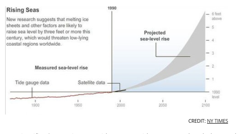
How Much Will It Cost to Solve Climate Change?

Switching from fossil fuels to low-carbon sources of energy will cost $44 trillion between now and 2050, according to a report released this week by the International Energy Agency.

Natural Gas and Fracking

How The Russia-China Gas Deal Hurts U.S. Liquid Natural Gas Industry

This could dampen the demand – and ultimately the price for – LNG from the United States. East Asia represents the most prized market for producers of LNG. That’s because it is home to the top three importers of LNG in the world: Japan, South Korea and China. Together, the three countries account for more than half of LNG demand worldwide. As a result, prices for LNG are as much as four to five times higher in Asia compared to what natural gas is sold for in the United States.

The Russia-China deal may change that.

If LNG prices in Asia come down from their recent highs, the most expensive LNG projects may no longer be profitable. That could force out several of the U.S. LNG projects waiting for U.S. Department of Energy approval. As of April, DOE had approved seven LNG terminals, but many more are waiting for permits.

LNG terminals in the United States will also not be the least expensive producers. The construction of several liquefaction facilities in Australia is way ahead of competitors in the U.S., and the country plans on nearly quadrupling its LNG capacity by 2017. More supplies and lower-than-expected demand from China could bring down prices over the next several years.

Write-down of two-thirds of US shale oil explodes fracking mythThis is big!

Next month, the US Energy Information Administration (EIA) will publish a new estimate of US shale deposits set to deal a death-blow to industry hype about a new golden era of US energy independence by fracking unconventional oil and gas.

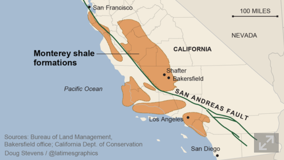
EIA officials told the Los Angeles Times that previous estimates of recoverable oil in the Monterey shale reserves in California of about 15.4 billion barrels were vastly overstated. The revised estimate, they said, will slash this amount by 96% to a puny 600 million barrels of oil.

The Monterey formation, previously believed to contain more than double the amount of oil estimated at the Bakken shale in North Dakota, and five times larger than the Eagle Ford shale in South Texas, was slated to add up to 2.8 million jobs by 2020 and boost government tax revenues by $24.6 billion a year.

China

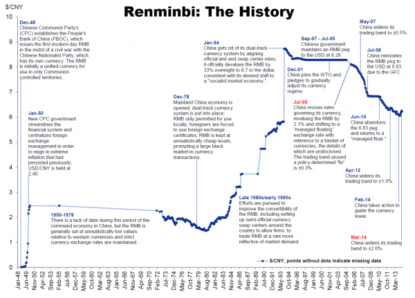
The Annotated History Of The World’s Next Reserve Currency

yuanhistory

Goldman: Prepare for Chinese property bust

…With demand poised to slow given a tepid economic backdrop, weaker household affordability, rising mortgage rates and developer cash flow weakness, we believe current construction capacity of the domestic property industry may be excessive. We estimate an inventory adjustment cycle of two years for developers, driving 10%-15% price cuts in most cities with 15% volume contraction from 2013 levels in 2014E-15E. We also expect M&A activities to take place actively, favoring developers with strong balance sheet and cash flow discipline.

China’s Shadow Banking Sector Valued At 80% of GDP

The China Banking Regulatory Commission has shed light on the country’s opaque shadow banking sector. It was as large as 33 trillion yuan ($5.29 trillion) in mid-2013 and equivalent to 80% of last year’s GDP, according to Yan Qingmin, a vice chairman of the commission.

In a Tuesday WeChat blog sent by the Chong Yang Institute for Financial Studies, Renmin University, Yan wrote that his calculation is based on shadow lending activities from asset management businesses to trust companies, a definition he said was very broad.  Yan said the rapid expansion of the sector, which was equivalent to 53% of GDP in 2012, entailed risks of some parts of the shadow banking business, but not necessarily the Chinese economy.

Yan’s estimation is notably higher than that of the Chinese Academy of Social Sciences. The government think tank said on May 9 that the sector has reached 27 trillion yuan ($4.4 trillion in 2013) and is equivalent to nearly one fifth of the domestic banking sector’s total assets.

Massive, Curvaceous Buildings Designed to Imitate a Mountain Forest

Chinamassive

Information Technology (IT)

I am an IT generalist. Am I doomed to low pay forever? Interesting comments and suggestions to this question on a Forum maintained by The Register.

I’m an IT generalist. I know a bit of everything – I can behave appropriately up to Cxx level both internally and with clients, and I’m happy to crawl under a desk to plug in network cables. I know a little bit about how nearly everything works – enough to fill in the gaps quickly: I didn’t know any C# a year ago, but 2 days into a project using it I could see the offshore guys were writing absolute rubbish. I can talk to DB folks about their DBs; network guys about their switches and wireless networks; programmers about their code and architects about their designs. Don’t get me wrong, I can do as well as talk, programming, design, architecture – but I would never claim to be the equal of a specialist (although some of the work I have seen from the soi-disant specialists makes me wonder whether I’m missing a trick).

My principle skill, if there is one – is problem resolution, from nitty gritty tech details (performance and functionality) to handling tricky internal politics to detoxify projects and get them moving again.

How on earth do I sell this to an employer as a full-timer or contractor? Am I doomed to a low income role whilst the specialists command the big day rates? Or should I give up on IT altogether

Crowdfunding is brutal… even when it works

China bans Windows 8

China has banned government use of Windows 8, Microsoft Corp’s latest operating system, a blow to a US technology company that has long struggled with sales in the country.

The Central Government Procurement Center issued the ban on installing Windows 8 on Chinese government computers as part of a notice on the use of energy-saving products, posted on its website last week.

Data Analytics

Statistics of election irregularities – good forensic data analytics.

Russia and Energy – Some Geopolitics

A couple of charts highlight the dominant position Russia holds with respect to energy, and, specifically, specifically, natural gas production.

First, there is this trade graphic from the BP Statistical Review of World Energy 2013.

naturalgastrades

Clearly, Russia has dominant global position in natural gas trades.

The Europeans are primary consumers for Russian natural gas, and there are some significant dependencies, as this graphic shows.

Ukrainegas

So Russia’s position as a major energy supplier no doubt is operating as a constraint on sanctions for the annexation of Crimea.

On the other  hand, this is a mutual dependency. The US Energy Information Agency, for example, reports that oil and gas revenues accounted for 52% of federal budget revenues and over 70% of total exports in 2012.