Category Archives: predictive analytics

Perspectives

Blogging gets to be enjoyable, although demanding. It’s a great way to stay in touch, and probably heightens personal mental awareness, if you do it enough.

The “Business Forecasting” focus allows for great breadth, but may come with political constraints.

On this latter point, I assume people have to make a living. Populations cannot just spend all their time in mass rallies, and in political protests – although that really becomes dominant at certain crisis points. We have not reached one of those for a long time in the US, although there have been mobilizations throughout the Mid-East and North Africa recently.

Nate Silver brought forth the “hedgehog and fox” parable in his best seller – The Signal and the Noise. “The fox knows many things, but the hedgehog knows one big thing.”

My view is that business and other forecasting endeavors should be “fox-like” – drawing on many sources, including, but not limited to quantitative modeling.

What I Think Is Happening – Big Picture

Global dynamics often are directly related to business performance, particularly for multinationals.

And global dynamics usually are discussed by regions – Europe, North America, Asia-Pacific, South Asia, the Mid-east, South American, Africa.

The big story since around 2000 has been the emergence of the People’s Republic of China as a global player. You really can’t project the global economy without a fairly detailed understanding of what’s going on in China, the home of around 1.5 billion persons (not the official number).

Without delving much into detail, I think it is clear that a multi-centric world is emerging. Growth rates of China and India far surpass those of the United States and certainly of Europe – where many countries, especially those along the southern or outer rim – are mired in high unemployment, deflation, and negative growth since just after the financial crisis of 2008-2009.

The “old core” countries of Western Europe, the United States, Canada, and, really now, Japan are moving into a “post-industrial” world, as manufacturing jobs are outsourced to lower wage areas.

Layered on top of and providing support for out-sourcing, not only of manufacturing but also skilled professional tasks like computer programming, is an increasingly top-heavy edifice of finance.

Clearly, “the West” could not continue its pre-World War II monopoly of science and technology (Japan being in the pack here somewhere). Knowledge had to diffuse globally.

With the GATT (General Agreement on Tariffs and Trade) and the creation of the World Trade Organization (WTO) the volume of trade expanded with reduction on tariffs and other barriers (1980’s, 1990’s, early 2000’s).

In the United States the urban landscape became littered with “Big Box stores” offering shelves full of clothing, electronics, and other stuff delivered to the US in the large shipping containers you see stacked hundreds of feet high at major ports, like San Francisco or Los Angeles.

There is, indeed, a kind of “hollowing out” of the American industrial machine.

Possibly it’s only the US effort to maintain a defense establishment second-to-none and of an order of magnitude larger than anyone elses’ that sustains certain industrial activities shore-side. And even that is problematical, since the chain of contracting out can be complex and difficult and costly to follow, if you are a US regulator.

I’m a big fan of post-War Japan, in the sense that I strongly endorse the kinds of evaluations and decisions made by the Japanese Ministry of International Trade and Investment (MITI) in the decades following World War II. Of course, a nation whose industries and even standing structures lay in ruins has an opportunity to rebuild from the ground up.

In any case, sticking to a current focus, I see opportunities in the US, if the political will could be found. I refer here to the opportunity for infrastructure investment to replace aging bridges, schools, seaport and airport facilities.

In case you had not noticed, interest rates are almost zero. Issuing bonds to finance infrastructure could not face more favorable terms.

Another option, in my mind – and a hat-tip to the fearsome Walt Rostow for this kind of thinking – is for the US to concentrate its resources into medicine and medical care. Already, about one quarter of all spending in the US goes to health care and related activities. There are leading pharma and biotech companies, and still a highly developed system of biomedical research facilities affiliated with universities and medical schools – although the various “austerities” of recent years are taking their toll.

So, instead of pouring money down a rathole of chasing errant misfits in the deserts of the Middle East, why not redirect resources to amplify the medical industry in the US? Hospitals, after all, draw employees from all socioeconomic groups and all ethnicities. The US and other national populations are aging, and will want and need additional medical care. If the world could turn to the US for leading edge medical treatment, that in itself could be a kind of foreign policy, for those interested in maintaining US international dominance.

Tangential Forces

While writing in this vein, I might as well offer my underlying theory of social and economic change. It is that major change occurs primarily through the impact of tangential forces, things not fully seen or anticipated. Perhaps the only certainty about the future is that there will be surprises.

Quite a few others subscribe to this theory, and the cottage industry in alarming predictions of improbable events – meteor strikes, flipping of the earth’s axis, pandemics – is proof of this.

Really, it is quite amazing how the billions on this planet manage to muddle through.

But I am thinking here of climate change as a tangential force.

And it is also a huge challenge.

But it is a remarkably subtle thing, not withstanding the on-the-ground reality of droughts, hurricanes, tornados, floods, and so forth.

And it is something smack in the sweet spot of forecasting.

There is no discussion of suitable responses to climate change without reference to forecasts of global temperature and impacts, say, of significant increases in sea level.

But these things take place over many years and, then, boom a whole change of regime may be triggered – as ice core and other evidence suggests.

Flexibility, Redundancy, Avoidance of Over-Specialization

My brother (by a marriage) is a priest, formerly a tax lawyer. We have begun a dialogue recently where we are looking for some basis for a new politics and new outlook, really that would take the increasing fragility of some of our complex and highly specialized systems into account – creating some backup systems, places, refuges, if you will.

I think there is a general principle that we need to empower people to be able to help themselves – and I am not talking about eliminating the social safety net. The ruling groups in the United States, powerful interests, and politicians would be well advised to consider how we can create spaces for people “to do their thing.” We need to preserve certain types of environments and opportunities, and have a politics that speaks to this, as well as to how efficiency is going to be maximized by scrapping local control and letting global business from wherever come in and have its way – no interference allowed.

The reason Reid and I think of this as a search for a new politics is that, you know, the counterpoint is that all these impediments to getting the best profits possible just result in lower production levels, meaning then that you have not really done good by trying to preserve land uses or local agriculture, or locally produced manufactures.

I got it from a good source in Beijing some years ago that the Chinese Communist Party believes that full-out growth of production, despite the intense pollution, should be followed for a time, before dealing with that problem directly. If anyone has any doubts about the rationality of limiting profits (as conventionally defined), I suggest they spend some time in China during an intense bout of urban pollution somewhere.

Maybe there are abstract, theoretical tools which could be developed to support a new politics. Why not, for example, quantify value experienced by populations in a more comprehensive way? Why not link achievement of higher value differently measured with direct payments, somehow? I mean the whole system of money is largely an artifact of cyberspace anyway.

Anyway – takeaway thought, create spaces for people to do their thing. Pretty profound 21st Century political concept.

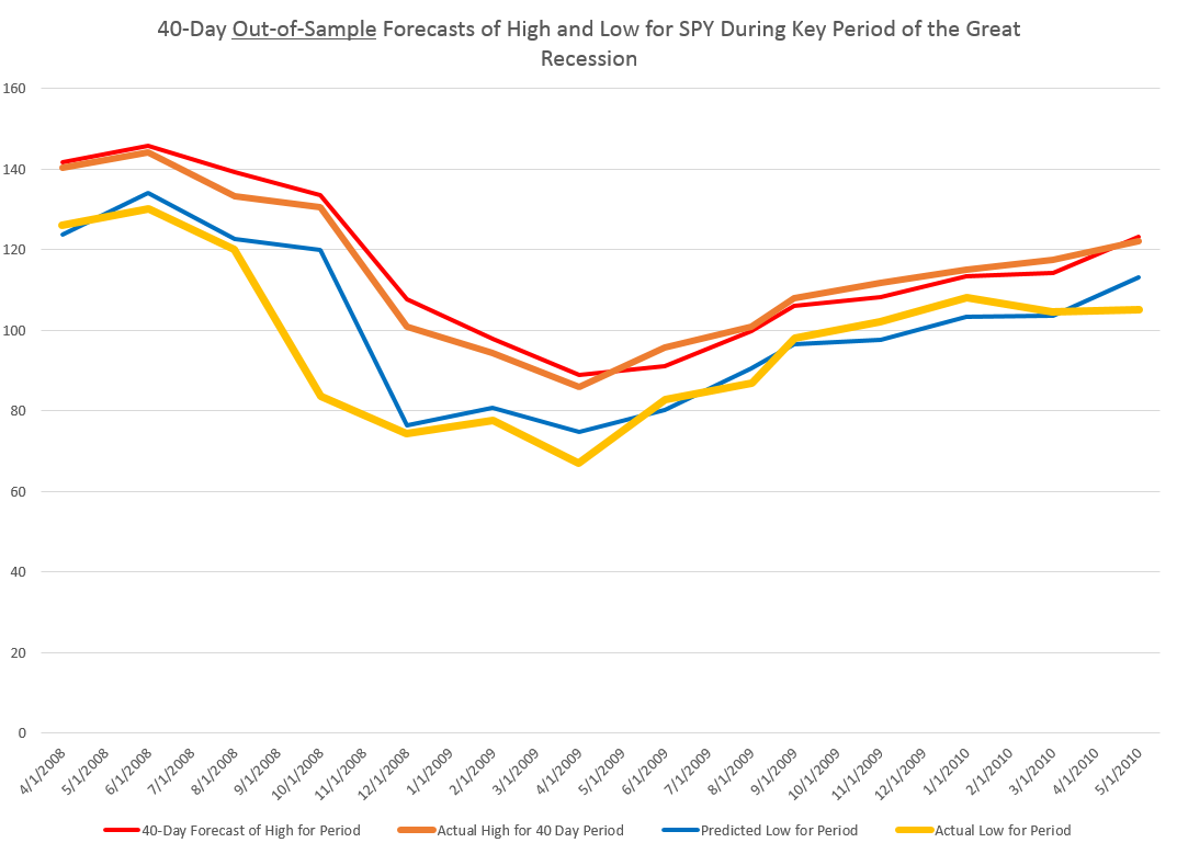
Coming attractions here – more on predicting the stock market (a new approach), summaries of outlooks for the year by major sources (banks, government agencies, leading economists), megatrends, forecasting controversies.

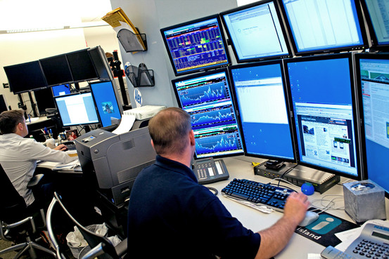
Top picture from FIREBELLY marketing

Trading Volume- Trends, Forecasts, Predictive Role

The New York Stock Exchange (NYSE) maintains a data library with historic numbers on trading volumes. Three charts built with some of this data tell an intriguing story about trends and predictability of volumes of transactions and dollars on the NYSE.

First, the number of daily transactions peaked during the financial troubles of 2008, only showing some resurgence lately.

transvol

This falloff in the number of transactions is paralleled by the volume of dollars spent in these transactions.

dollartrans

These charts are instructive, since both highlight the existence of “spikes” in transaction and dollar volume that would seem to defy almost any run-of-the-mill forecasting algorithm. This is especially true for the transactions time series, since the spikes are more irregularly spaced. The dollar volume time series suggests some type of periodicity is possible for these spikes, particularly in recent years.

But lower trading volume has not impacted stock prices, which, as everyone knows, surged past 2008 levels some time ago.

A raw ratio between the value of trades and NYSE stock transactions gives the average daily price per transaction.

vluepershare

So stock prices have rebounded, for the most part, to 2008 levels. Note here that the S&P 500 index stocks have done much better than this average for all stocks.

Why has trading volume declined on the NYSE? Some reasons gleaned from the commentariat.

  1. Mom and Pop traders largely exited the market, after the crash of 2008
  2. Some claim that program trading or high frequency trading peaked a few years back, and is currently in something of a decline in terms of its proportion of total stock transactions. This is, however, not confirmed by the NYSE Facts and Figures, which shows program trading pretty consistently at around 30 percent of total trading transactions..
  3. Interest has shifted to options and futures, where trading volumes are rising.
  4. Exchange Traded Funds (ETF’s) make up a larger portion of the market, and they, of course, do not actively trade.
  5. Banks have reduced their speculation in equities, in anticipation of Federal regulations

See especially Market Watch and Barry Ritholtz on these trends.

But what about the impact of trading volume on price? That’s the real zinger of a question I hope to address in coming posts this week.

How Did My Forecast of the SPY High and Low Issued January 22 Do?

A couple of months ago, I applied the stock market forecasting approach based on what I call “proximity variables” to forward-looking forecasts – as opposed to “backcasts” testing against history.

I’m surprised now that I look back at this, because I offered a forecast for 40 trading days (a little foolhardy?).

In any case, I offered forecasts for the high and low of the exchange traded fund SPY, as follows:

What about the coming period of 40 trading days, starting from this morning’s (January 22, 2015) opening price for the SPY – $203.99?

Well, subject to qualifications I will state further on here, my estimates suggest the high for the period will be in the range of $215 and the period low will be around $194. Cents attached to these forecasts would be, of course, largely spurious precision.

In my opinion, these predictions are solid enough to suggest that no stock market crash is in the cards over the next 40 trading days, nor will there be a huge correction. Things look to trade within a range not too distant from the current situation, with some likelihood of higher highs.

It sounds a little like weather forecasting.

Well, 27 trading days have transpired since January 22, 2015 – more than half the proposed 40 associated with the forecast.

How did I do?

Here is a screenshot of the Yahoo Finance table showing opening, high, low, and closing prices since January 22, 2015.

SPYJan22etpassim

The bottom line – so far, so good. Neither the high nor low of any trading day has broached my proposed forecasts of $194 for the low and $215 for the high.

Now, I am pleased – a win just out of the gates with the new modeling approach.

However, I would caution readers seeking to use this for investment purposes. This approach recommends shorter term forecasts to focus in on the remaining days of the original forecast period. So, while I am encouraged the $215 high has not been broached, despite the hoopla about recent gains in the market, I don’t recommend taking $215 as an actual forecast at this point for the remaining 13 trading days – two or three weeks. Better forecasts are available from the model now.

“What are they?”

Well, there are a lot of moving parts in the computer programs to make these types of updates.

Still, it is interesting and relevant to forecasting practice – just how well do the models perform in real time?

So I am planning a new feature, a periodic update of stock market forecasts, with a look at how well these did. Give me a few days to get this up and running.

Modeling High Tech – the Demand for Communications Services

A colleague was kind enough to provide me with a copy of –

Demand for Communications Services – Insights and Perspectives, Essays in Honor of Lester D. Taylor, Alleman, NíShúilleabháin, and Rappoport, editors, Springer 2014

Some essays in this Festschrift for Lester Taylor are particularly relevant, since they deal directly with forecasting the disarray caused by disruptive technologies in IT markets and companies.

Thus, Mohsen Hamoudia in “Forecasting the Demand for Business Communications Services” observes about the telecom space that

“..convergence of IT and telecommunications market has created more complex behavior of market participants. Customers expect new product offerings to coincide with these emerging needs fostered by their growth and globalization. Enterprises require more integrated solutions for security, mobility, hosting, new added-value services, outsourcing and voice over internet protocol (VoiP). This changing landscape has led to the decline of traditional product markets for telecommunications operators.

In this shifting landscape, it is nothing less than heroic to discriminate “demand variables” and “ independent variables” deploying and produce useful demand forecasts from three stage least squares (3SLS) models, as does Mohsen Hamoudia in his analysis of BCS.

Here is Hamoudia’s schematic of supply and demand in the BCS space, as of a 2012 update.

BCS

Other cutting-edge contributions, dealing with shifting priorities of consumers, faced with new communications technologies and services, include, “Forecasting Video Cord-Cutting: The Bypass of Traditional Pay Television” and “Residential Demand for Wireless Telephony.”

Festschrift and Elasticities

This Springer Festschrift is distinctive inasmuch as Professor Taylor himself contributes papers – one a reminiscence titled “Fifty Years of Studying Economics.”

Taylor, of course, is known for his work in the statistical analysis of empirical demand functions and broke ground with two books, Telecommunications Demand: A Survey and Critique (1980) and Telecommunications Demand in Theory and Practice (1994).

Accordingly, forecasting and analysis of communications and high tech are a major focus of several essays in the book.

Elasticities are an important focus of statistical demand analysis. They flow nicely from double logarithmic or log-log demand specifications – since, then, elasticities are constant. In a simple linear demand specification, of course, the price elasticity varies across the range of prices and demand, which complicates testimony before public commissions, to say the least.

So it is interesting, in this regard, that Professor Taylor is still active in modeling, contributing to his own Festschrift with a note on translating logs of negative numbers to polar coordinates and the complex plane.

“Pricing and Maximizing Profits Within Corporations” captures the flavor of a telecom regulatory era which is fast receding behind us. The authors, Levy and Tardiff, write that,

During the time in which he was finishing the update, Professor Taylor participated in one of the most hotly debated telecommunications demand elasticity issues of the early 1990’s: how price-sensitive were short-distance toll calls (then called intraLATA long-distance calls)? The answer to that question would determine the extent to which the California state regulator reduced long-distance prices (and increased other prices, such as basic local service prices) in a “revenue-neutral” fashion.

Followup Workshop

Research in this volume provides a good lead-up to a forthcoming International Institute of Forecasters (IIF) workshop – the 2nd ICT and Innovation Forecasting Workshop to be held this coming May in Paris.

The dynamic, ever changing nature of the Information & Communications Technology (ICT) Industry is a challenge for business planners and forecasters. The rise of Twitter and the sudden demise of Blackberry are dramatic examples of the uncertainties of the industry; these events clearly demonstrate how radically the environment can change. Similarly, predicting demand, market penetration, new markets, and the impact of new innovations in the ICT sector offer a challenge to businesses and policymakers. This Workshop will focus on forecasting new services and innovation in this sector as well as the theory and practice of forecasting in the sector (Telcos, IT providers, OTTs, manufacturers). For more information on venue, organizers and registration, Download brochure

High Frequency Trading – 2

High Frequency Trading (HFT) occurs faster than human response times – often quoted as 750 milliseconds. It is machine or algorithmic trading, as Sean Gourley’s “High Frequency Trading and the New Algorithmic Ecosystem” highlights.

This is a useful introductory video.

It mentions Fixnetix’s field programmable array chip and new undersea cables designed to shave milliseconds off trading speeds from Europe to the US and elsewhere.

Also, Gourley refers to dark pool pinging, which tries to determine the state of large institutional orders by “sniffing them out” and using this knowledge to make (almost) risk-free arbitrage by trading on different exchanges in milliseconds or faster. Institutional investors using slower and not-so-smart algorithms lose.

Other HFT tractics include “quote stuffing”, “smoking”, and “spoofing.” Of these, stuffing may be the most damaging. It limits access of slower traders by submitting large numbers of orders and then canceling them very quickly. This leads to order congestion, which may create technical trouble and lagging quotes.

Smoking and spoofing strategies, on the other hand, try to manipulate other traders to participate in trading at unfavorable moments, such as just before the arrival of relevant news.

Here are some more useful links on this important development and the technological arms race that has unfolded around it.

Financial black swans driven by ultrafast machine ecology Key research on ultrafast black swan events

Nanosecond Trading Could Make Markets Go Haywire Excellent Wired article

High-Frequency Trading and Price Discovery

Defense of HFT on basis that HFTs’ trade (buy or sell) in the direction of permanent price changes and against transitory pricing errors creates benefits which outweigh adverse selection of HFT liquidity supplying (non-marketable) limit orders.

The Good, the Bad, and the Ugly of Automated High-Frequency Trading tries to strike a balance, but tilts toward a critique

Has HFT seen its heyday? I read at one and the same time I read at one and the same time that HFT profits per trade are dropping, that some High Frequency Trading companies report lower profits or are shutting their doors, but that 70 percent of the trades on the New York Stock Exchange are the result of high frequency trading.

My guess is that HFT is a force to be dealt with, and if financial regulators are put under restraint by the new US Congress, we may see exotic new forms flourishing in this area. 

Forecasting the S&P 500 – Short and Long Time Horizons

Friends and acquaintances know that I believe I have discovered amazing, deep, and apparently simple predictability in aspects of the daily, weekly, monthly movement of stock prices.

People say – “don’t blog about it, keep it to yourself, and use it to make a million dollars.” That does sound attractive, but I guess I am a data scientist, rather than stock trader. Not only that, but the pattern looks to be self-fulfilling. Generally, the result of traders learning about this pattern should be to reinforce, rather than erase, it. There seems to be no other explanation consistent with its long historical vintage, nor the broadness of its presence. And that is big news to those of us who like to linger in the forecasting zoo.

I am going to share my discovery with you, at least in part, in this blog post.

But first, let me state some ground rules and describe the general tenor of my analysis. I am using OLS regression in spreadsheets at first, to explore the data. I am only interested, really, in models which have significant out-of-sample prediction capabilities. This means I estimate the regression model over a set of historical data and then use that model to predict – in this case the high and low of the SPY exchange traded fund. The predictions (or “retrodictions” or “backcasts”) are for observations on the high and low stock prices for various periods not included in the data used to estimate the model.

Now let’s look at the sort of data I use. The following table is from Yahoo Finance for the SPY. The site allows you to download this data into a spreadsheet, although you have to invert the order of the dating with a sort on the date. Note that all data is for trading days, and when I speak of N-day periods in the following, I mean periods of N trading days.

Yahoo

OK, now let me state my major result.

For every period from daily periods to 60 day periods I have investigated, the high and low prices are “relatively” predictable and the direction of change from period to period is predictable, in backcasting analysis, about 70-80 percent of the time, on average.

To give an example of a backcasting analysis, consider this chart from the period of free-fall in markets during 2008-2009, the Great Recession (click to enlarge).

40dayforecast

Now note that the indicated lines for the forecasts are not, strictly-speaking, 40-day-ahead forecasts. The forecasts are for the level of the high and low prices of the SPY which will be attained in each period of 40 trading days.

But the point is these rather time-indeterminate forecasts, when graphed alongside the actual highs and lows for the 40 trading day periods in question, are relatively predictive.

More to the point, the forecasts suffice to signal a key turning point in the SPY. Of course, it is simple to relate the high and low of the SPY for a period to relevant measures of the average or closing stock prices.

So seasoned forecasters and students of the markets and economics should know by this example that we are in terra incognita. Forecasting turning points out-of-sample is literally the toughest thing to do in forecasting, and certain with respect to the US stock market.

Many times technical analysts claim to predict turning points, but their results may seem more artistic, involving subtle interpretations of peaks and shoulders, as well as levels of support.

Now I don’t want to dismiss technical analysis, since, indeed, I believe my findings may prove out certain types of typical results in technical analysis. Or at least I can see a way to establish that claim, if things work out empirically.

Forecast of SPY High And Low for the Next Period of 40 Trading Days

What about the coming period of 40 trading days, starting from this morning’s (January 22, 2015) opening price for the SPY – $203.99?

Well, subject to qualifications I will state further on here, my estimates suggest the high for the period will be in the range of $215 and the period low will be around $194. Cents attached to these forecasts would be, of course, largely spurious precision.

In my opinion, these predictions are solid enough to suggest that no stock market crash is in the cards over the next 40 trading days, nor will there be a huge correction. Things look to trade within a range not too distant from the current situation, with some likelihood of higher highs.

It sounds a little like weather forecasting.

The Basic Model

Here is the actual regression output for predicting the 40 trading day high of the SPY.

40Highreg

This is a simpler than many of the models I have developed, since it only relies on one explanatory variable designated X Variable 1 in the Excel regression output. This explanatory variable is the ratio of the current opening price to the previous high for the 40 day trading period, all minus 1.

Let’s call this -1+ O/PH. Instances of -1+ O/PH are generated for data bunched by 40 trading day periods, and put into the regression against the growth in consecutive highs for these 40 day periods.

So what happens is this, apparently.

Everything depends on the opening price. If the high for the previous period equals the opening price, the predicted high for the next 40 day period will be the same as the high for the previous 40 day period.

If the previous high is less than the opening price, the prediction is that the next period high will be higher. Otherwise, the prediction is that the next period high will be lower.

This then looks like a trading rule which even the numerically challenged could follow.

And this sort of relationship is not something that has just emerged with quants and high frequency trading. On the contrary, it is possible to find the same type of rule operating with, say, Exxon’s stock (XOM) in the 1970’s and 1980’s.

But, before jumping to test this out completely, understand that the above regression is, in terms of most of my analysis, partial, missing at least one other important explanatory variable.

Previous posts, which employ similar forecasting models for daily, weekly, and monthly trading periods, show that these models can predict the direction of change of the period highs with about 70 to 80 percent accuracy (See, for example, here).

Provisos and Qualifications

In deploying OLS regression analysis, in Excel spreadsheets no less, I am aware there are many refinements which, logically, might be developed and which may improve forecast accuracy.

One thing I want to stress is that residuals of the OLS regressions on the growth in the period highs generally are not normally distributed. The distribution tends to be very peaked, reminiscent of discussions earlier in this blog of the Laplace distribution for Microsoft stock prices.

There also is first order serial correlation in many of these regressions. And, my software indicates that there could be autocorrelations extending deep into the historical record.

Finally, the regression coefficients may vary over the historical record.

Bottom LIne

I like Robb Hyndman’s often drawn distinction between modeling and reality. Somewhere Hyndman suggests that no model is right.

But this class of models has an extremely logical motivation, and is, as I say, relatively predictive – predictive enough to be useful in a number of contexts.

Momentum traders for years apparently have looked at the opening price and compared it with the highs (and lows) for previous periods – extending 60 days or more into history if not more – and decided whether to trade. If the opening price is greater than the past high, the next high is anticipated to be even higher. On this basis, stock may be purchased. That action tends to reinforce the relationship. So, in some sense, this is a self-fulfilling relationship.

To recapitulate – I can show you iron-clad, incontrovertible evidence that some fairly simple models built on daily trading data produce workable forecasts of the high and low for stock indexes and stocks. These forecasts are available for a variety of time periods, and, apparently, in backcasts can indicate turning points in the market.

As I say, feel free to request further documentation. I am preparing a write-up for a journal, and I think I can find a way to send out versions of this.

You can contact me confidentially via the Comments box below. Leave your email or phone number. Title the Comment “Request for High/Low Model Information” and the webmeister will forward it to me without having your request listed in the side panel of the blog.

Updates on Forecasting Controversies – Google Flu Trends

Last Spring I started writing about “forecasting controversies.”

A short list of these includes Google’s flu forecasting algorithm, impacts of Quantitative Easing, estimates of energy reserves in the Monterey Shale, seasonal adjustment of key series from Federal statistical agencies, and China – Trade Colossus or Assembly Site?

Well, the end of the year is a good time to revisit these, particularly if there are any late-breaking developments.

Google Flu Trends

Google Flu Trends got a lot of negative press in early 2014. A critical article in Nature – When Google got flu wrong – kicked it off. A followup Times article used the phrase “the limits of big data,” while the Guardian wrote of Big Data “hubris.”

The problem was, as the Google Trends team admits –

In the 2012/2013 season, we significantly overpredicted compared to the CDC’s reported U.S. flu levels.

Well, as of October, Google Flu Trends has a new engine. This like many of the best performing methods … in the literature—takes official CDC flu data into account as the flu season progresses.

Interestingly, the British Royal Society published an account at the end of October – Adaptive nowcasting of influenza outbreaks using Google searches – which does exactly that – merges Google Flu Trends and CDC data, achieving impressive results.

The authors develop ARIMA models using “standard automatic model selection procedures,” citing a 1998 forecasting book by Hyndman, Wheelwright, and Makridakis and a recent econometrics text by Stock and Watson. They deploy these adaptively-estimated models in nowcasting US patient visits due to influenza-like illnesses (ILI), as recorded by the US CDC.

The results are shown in the following panel of charts.

GoogleFluTrends

Definitely click on this graphic to enlarge it, since the key point is the red bars are the forecast or nowcast models incorporating Google Flu Trends data, while the blue bars only utilize more conventional metrics, such as those supplied by the Centers for Disease Control (CDC). In many cases, the red bars are smaller than the blue bar for the corresponding date.

The lower chart labeled ( c ) documents out-of-sample performance. Mean Absolute Error (MAE) for the models with Google Flu Trends data are 17 percent lower.

It’s relevant , too, that the authors, Preis and Moat, utilize unreconstituted Google Flu Trends output – before the recent update, for example – and still get highly significant improvements.

I can think of ways to further improve this research – for example, deploy the Hyndman R programs to automatically parameterize the ARIMA models, providing a more explicit and widely tested procedural referent.

But, score one for Google and Hal Varian!

The other forecasting controversies noted above are less easily resolved, although there are developments to mention.

Stay tuned.

Predicting the Midterm Elections

Predicting the outcome of elections is a fascinating game with more and more sophisticated predictive analytics.

The Republicans won bigtime, of course.

They won comfortable control of the US Senate and further consolidated their majority in the House of Representatives.

Counting before the Louisiana runoff election, which a Republican is expected to win, the balance is 52 to 44 in the Senate, highlighted in the following map from Politico.

senateresults

In the US House of Representatives, Republicans gained 12 seats for a 57 percent majority, 244 to 184, as illustrated in a New York Times graphic.

houseresults

Did Anyone See This Coming?

Nate Silver, who was prescient in the 2012 General Election, issued an update on his website FiveThirtyEight on November 4 stating that Republicans Have A 3 In 4 Chance Of Winning The Senate.

And so they did win.

Salon’s review of Silver’s predictions notes that,

Overall, the candidate with better-than-even odds in FiveThirtyEight’s model won or is likely to in 34 of the 36 Senate contests this year, for a success rate of 94 percent.

The track record for the governorships was less shining, with upsets in Maryland and Kansas and several wins by candidates with unfavorable odds in the FiveThirtyEight lineup.

Bias in Polls

Silver’s forecasting model weighs both polling data and fundamentals- like demographics.

After the election, Silver blamed some of his mistakes on bias in polls, claiming that, this time, the Polls Were Skewed Toward Democrats.

Based on results as reported through early Wednesday morning …. the average Senate poll conducted in the final three weeks of this year’s campaign overestimated the Democrat’s performance by 4 percentage points. The average gubernatorial poll was nearly as bad, overestimating the Democrat’s performance by 3.4 points.

He backs this up with details of bias in polls by race, and, interestingly, throws up the following exhibit, suggesting that there is nothing systematic about bias in the polls.

biaspolls

Here is another discussion of mid-term election polling error – arguing it is significantly greater during midterms than in Presidential election years.

While not my area of expertise (although I have designed and analyzed survey data), I’m think the changing demographics of “cell-only” voters, no-call lists, and people’s readiness to hang up on unsolicited calls impacts the reliability of polling data, as usually gathered. What Silver seems to show with his graphic above, is that adjusting for these changes causes another form of unreliability.

Speculators and Oil Prices

One of the more important questions in the petroleum business is the degree to which speculators influence oil prices.

CrudeOilSpotPrice

If speculators can significantly move oil spot prices, there might be “overshooting” on the downside, in the current oil price environment. That is, the spot price of oil might drop more than fundamentals warrant, given that spot prices have dropped significantly in recent weeks and the Saudi’s may not reduce production, as they have in the past.

This issue can be rephrased more colorfully in terms of whether the 2008 oil price spike, shown below, was a “bubble,” driven in part by speculators, or whether, as some economists argue, things can be explained in terms of surging Chinese demand and supply constraints.

James Hamilton’s Causes and Consequences of the Oil Shock of 2007–08, Spring 2009, documents a failure of oil production to increase between 2005-2007, and the exponential growth in Chinese petroleum demand through 2007.

Hamilton, nevertheless, admits “the speed and magnitude of the price collapse leads one to give serious consideration to the alternative hypothesis that this episode represents a speculative price bubble that popped.”

Enter hedge fund manager Michael Masters stage left.

In testimony before the US Senate, Masters blames the 2007-08 oil price spike on speculators, and specifically on commodity index trading funds which held a quarter trillion dollars worth of futures contracts in 2008.

Hamilton characterizes Masters’ position as follows,

A typical strategy is to take a long position in a near-term futures contract, sell it a few weeks before expiry, and use the proceeds to take a long position in a subsequent near-term futures contract. When commodity prices are rising, the sell price should be higher than the buy, and the investor can profit without ever physically taking delivery. As more investment funds sought to take positions in commodity futures contracts for this purpose, so that the number of buys of next contracts always exceeded the number of sells of expiring ones, the effect, Masters argues, was to drive up the futures price, and with it the spot price. This “financialization” of commodities, according to Masters, introduced a speculative bubble in the price of oil.

Where’s the Beef?

If speculators were instrumental in driving up oil prices in 2008, however, where is the inventory build one would expect to accompany such activity? As noted above, oil production 2005-2007 was relatively static.

There are several possible answers.

One is simply that activity in the futures markets involve “paper barrels of oil” and that pricing of real supplies follows signals being generated by the futures markets. This is essentially Masters’ position.

A second, more sophisticated response is that the term structure of the oil futures markets changed, running up to 2008. The sweet spot changed from short term to long term futures, encouraging “ground storage,” rather than immediate extraction and stockpiling of inventories in storage tanks. Short term pricing followed the lead being indicated by longer term oil futures. The MIT researcher Parsons makes this case in a fascinating paper Black Gold & Fool’s Gold: Speculation in the Oil Futures Market.

..successful innovations in the financial industry made it possible for paper oil to be a financial asset in a very complete way. Once that was accomplished, a speculative bubble became possible. Oil is no different from equities or housing in this regard.

A third, more conventional answer is that, in fact, it is possible to show a direct causal link from activity in the oil futures markets to oil inventories, despite the appearances of flat production leading up to 2008.

Where This Leads

The uproar on this issue is related to efforts to increase regulation on the nasty speculators, who are distorting oil and other commodity prices away from values determined by fundamental forces.

While that might be a fine objective, I am more interested in the predictive standpoint.

Well, there is enough here to justify collecting a wide scope of data on production, prices, storage, reserves, and futures markets, and developing predictive models. It’s not clear the result would be most successful short term, or for the longer term. But I suspect forward-looking perspective is possible through predictive analytics in this area.

Top graphic from Evil Speculator.

Oil and Gas Prices II

One of the more interesting questions in applied forecasting is the relationship between oil and natural gas prices in the US market, shown below.

OIlGasPrices

Up to the early 1990’s, the interplay between oil and gas prices followed “rules of thumb” – for example, gas prices per million Btu were approximately one tenth oil prices.

There is still some suggestion of this – for example, peak oil prices recently hit nearly $140 a barrel, at the same time gas prices were nearly $14 per million Btu’s.

However, generally, ratio relationships appear to break down around 2009, if not earlier, during the first decade of the century.

A Longer Term Relationship?

Perhaps oil and gas prices are in a longer term relationship, but one disturbed in many cases in short run time periods.

One way economists and ecommetricians think of this is in terms of “co-integrating relationships.” That’s a fancy way of saying that regressions of the form,

Gas price in time t = constant + α(oil price in time t) + (residual in time t)

are predictive. Here, α is a coefficient to be estimated.

Now this looks like a straight-forward regression, so you might say – “what’s the problem?”

Well, the catch is that gas prices and oil prices might be nonstationary – that is, one or another form of a random walk.

If this is so – and positive results on standard tests such as the augmented Dickey Fuller (ADR) and Phillips-Peron are widely reported – there is a big potential problem. It’s easy to regress one completely unrelated nonstationary time series onto another, getting an apparently significant result, only to find this relationship disappears in the forecast. In other words two random series can, by chance, match up to each other over closely, but that’s no guarantee they will continue to do so.

Here’s where the concept of a co-integrating relationship comes into play.

If you can show, by various statistical tests, that variables are cointegrated, regressions such as the one above are more likely to be predictive.

Well, several econometric studies show gas and oil prices are in a cointegrated relationship, using data from the 1990’s through sometime in the first decade of the 2000’s. The more sophisticated specify auxiliary variables to account for weather or changes in gas storage. You might download and read, for example, a study published in 2007 under the auspices of the Dallas Federal Reserve Bank – What Drives Natural Gas Prices?

But it does not appear that this cointegrated relationship is fixed. Instead, it changes over time, perhaps exemplifying various regimes, i.e. periods of time in which the underlying parameters switch to new values, even though a determinate relationship can still be demonstrated.

Changing parameters are shown in the excellent 2012 study by Ramberg and Parsons in the Energy Journal – The Weak Tie Between Natural Gas and Oil Prices.

The Underlying Basis

Anyway, there are facts relating to production and use of oil and natural gas which encourage us to postulate a relationship in their prices, although the relationship may shift over time.

This makes sense since oil and gas are limited or completely substitutes in various industrial processes. This used to be more compelling in electric power generation, than it is today. According to the US Department of Energy, there are only limited amounts of electric power still produced by generators running on oil, although natural gas turbines have grown in importance.

Still, natural gas is often produced alongside of and is usually dissolved in oil, so oil and natural gas are usually joint products.

Recently, technology has changed the picture with respect to gas and oil.

On the demand side, the introduction of the combined-cycle combustion turbine made natural gas electricity generation more cost effective, thereby making natural gas in electric power generation even more dominant.

On the demand side, the new technologies of extracting shale oil and natural gas – often summarized under the rubric of “fracking” or hydraulic fracturing – have totally changed the equation, resulting in dramatic increases in natural gas supplies in the US.

This leaves the interesting question of what sort of forecasting model for natural gas might be appropriate.