
As I wrote recently, most business forecasting assignments are relatively simple. You collect the data (often the most challenging part), and plug this data into an automatic forecasting program. The program probably applies some type of exponential smoothing (ES) to produce forecasts for a horizon of a few periods ahead, and, bam, there you have it. The rest is presentation, developing the “story” and so forth.
So what about this exponential smoothing? What’s basically involved? What are the differences between exponential smoothing and the other primary univariate forecasting technique – ARIMA or Box-Jenkins modeling? What are these automatic forecasting programs, and which ones are best?
All good questions, and, if you are interested or involved in forecasting, the answers are good to rehearse from time to time.
Level, Trend, Seasonality – Components of Time Series
Exponential smoothing originated with the work of Brown and Holt for the US Navy (see the discussion in Gardiner). The perspective was not theoretical, but applied.
Nevertheless, there is an intuitive aspect to exponential smoothing (ES). That has to do with the decomposition of time series into components – such as level, trend, and seasonal effects.
So, applying the algorithms of ES to some time series Xt t=1,2,…,n, we extract estimates of the level Lt, trend Tt, and seasonal component, St, so that at any time t, we can express Xt as
Xt = Lt + Tt + St
This would be an additive model.
It’s also possible that the time series Xt could be multiplicative, as in
Xt = LtTtSt
By way of example, consider the following time series for public construction spending in the US, obtained from FRED (Federal Reserve Economic Data).
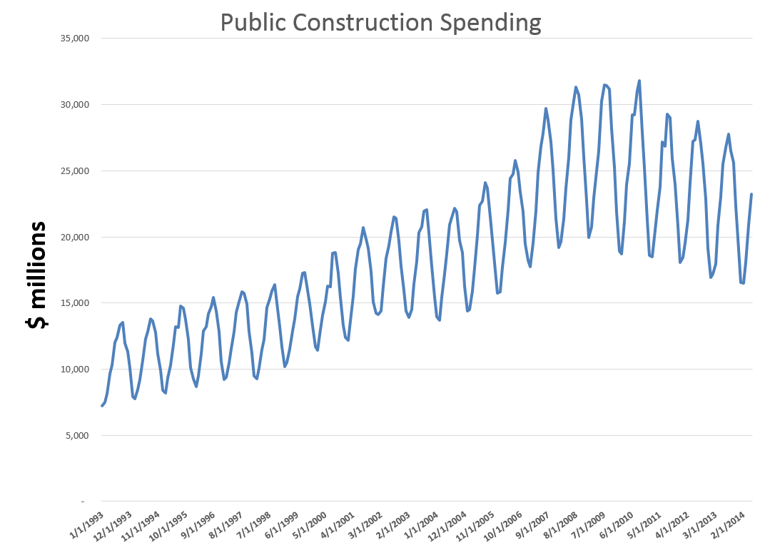
Now if you look closely, it’s clear there are strongly delineated seasonal effects. Furthermore, these seasonal variations appear to fluctuate more or less in proportion to the annual levels of the series. Thus, the variation is considerably more over a year, when spending is at a $25 billion level, than it does at a $10 billion level.
And the fact that these levels are different, and the series does not simply oscillate around a single level, indicates that there is probably a meaningful trend component to this time series.
Automatic Forecasting Programs
These are the considerations that you take into account in building an exponential smoothing model.
Now it is possible to create ES models within the framework of a spreadsheet. Thus, ES models have smoothing parameters which can be set by minimizing a squared sum of forecast errors over historic data. In Microsoft’s Excel, you can use Solver to do this, once you set up the recursion equations for level, trend, and seasonal components or effects.
In coming posts, I want to show how this can be done for a simple example.
But really, setting up spreadsheets to estimate exponential smoothing models can be laborious, since you need a separate set of computations for every possible model. In addition to the additive and purely multiplicative models shown above, for example, there can be hybrid cases – multiplicative seasonality but additive trend, and so forth.
So it’s a good idea to equip yourself with one of the several, good automatic forecasting programs out there to speed model identification and evaluation.
I will have reference to two such automatic forecasting programs in coming posts – Forecast Pro and Rob Hyndman’s Forecast package in R. I’ll make comparisons between these programs. A demo version of Forecast Pro is available for download for free, but it is a commercial package with various options at various price steps. Hyndman’s R forecasting package, on the other hand, is open source software and free, as is the R platform. While this sounds like an unbeatable advantage, there always are questions of bugs and performance – which in this case seem to be to be resolved for reasons we can discuss.
What’s The Big Deal?
Finally, the reason why ES forecasting is so widely applied is that, in many cases, it produces forecasts which are of comparable or superior accuracy to other univariate forecasting approaches.
ES has performed well, for example, in international forecasting competitions, including the widely-publicized M-competitions.
There also is a link between exponential smoothing and the Kalman filter. So ES is in a sense an adaptive forecasting approach. For example, ES weights more recent observations more heavily than observations more distant in the past, unlike a regression trend model.
Finally, recent research has provided statistical pedigree to exponential smoothing, rescuing it in a sense from consignment to “a purely ad hoc” approach. Thus, there is a direct link between time series that embody a random walk or random walk with drift and exponential smoothing.