Tag Archives: financial forecasts

More on Negative Nominal Interest Rates

The European Central Bank (ECB) experiment with negative interest rates has not occurred in a vacuum. The concept has been discussed with special urgency since 2008 in academic and financial circles.

Recently, Larry Summers and Paul Krugman have developed perspectives on the desirability of busting through the zero bound on interest rates to help balance aggregate demand and supply at something like full employment.

Then, there is Ken Rogoff’s Costs and Benefits to Phasing Out Paper Currency, distributed by the National Bureau of Economic Research (NBER).

Rogoff notes,

If all central bank liabilities were electronic, paying a negative interest on reserves (basically charging a fee) would be trivial. But as long as central banks stand ready to convert electronic deposits to zero-interest paper currency in unlimited amounts, it suddenly becomes very hard to push interest rates below levels of, say, -0.25 to -0.50 percent, certainly not on a sustained basis. Hoarding cash may be inconvenient and risky, but if rates become too negative, it becomes worth it.

Rogoff cites Buiter’s research at the London School of Economics (LSE) which dates to a decade earler, but has been significantly revised in the 2009-10 timeframe.

For example, there is Negative Nominal Interest Rates: Three ways to overcome the zero lower bound, which sports the following abstract:

The paper considers three methods for eliminating the zero lower bound on nominal interest rates and thus for restoring symmetry to domain over which the central bank can vary its policy rate. They are: (1) abolishing currency (which would also be a useful crime-fighting measure); (2) paying negative interest on currency by taxing currency; and (3) decoupling the numéraire from the currency/medium of exchange/means of payment and introducing an exchange rate between the numéraire and the currency which can be set to achieve a forward discount (expected depreciation) of the currency vis-a-vis the numéraire when the nominal interest rate in terms of the numéraire is set at a negative level for monetary policy purposes.

Buiter notes the “scrip” money developed locally during the Great Depression (also see Champ) effectively involved a tax on holding this type of currency.

Stamp scrip, sometimes called coupon scrip, arose in several communities. It was denominated in dollars, in denominations from 25 cents to $5, with $1 denominations most common. Stamp scrip often became redeemable by the issuer in official U.S. dollars after one year.

What made stamp scrip unique among scrip schemes was a series of boxes on the reverse side of the note. Stamp scrip took two basic forms—dated and undated (often called “transaction stamp scrip”). Typically, 52 boxes appeared on the back of dated stamp scrip, one for each week of the year. In order to spend the dated scrip, the stamps on the back had to be current. Each week, a two-cent stamp needed to be purchased from the issuer and affixed over the corresponding week’s box on the back of the scrip. Over the coming week, the scrip could be spent freely within the community. Whoever was caught holding the scrip at week’s end was required to attach a new stamp before spending the scrip. In this scheme, money became a hot potato, with individuals passing it quickly to avoid having to pay for the next stamp.

Among the virtues of eliminating paper currency and going entirely to electronic transactions, thus, would be that the central bank could charge a negative interest rate.

Additionally, by eliminating the anonymity of paper money and coin, criminal activities could be more effectively controlled. Rogoff offers calculations suggesting the percentages of US currency held in Europe in ratio to overall economic activity are suspicious, especially since there are apparently a surfeit of 100 dollar bills in these foreign holdings.

These ideas go considerably beyond the small negative interest charged by the ECB on banks holding excess reserves in the central bank accounts. What is being discussed is an extension of negative nominal interest, or a tax on holding cash, to all business agents and individuals in an economy.

Europe, the European Union, the Eurozone – Key Facts and Salient Issues

Considering that social and systems analysis originated largely in Europe (Machiavelli, Vico, Max Weber, Emile Durkheim, Walras, Adam Smith and the English school of political economics, and so forth), it’s not surprising that any deep analysis of the current European situation is almost alarmingly complex, reticulate, and full of nuance.

However, numbers speak for themselves, to an extent, and I want to start with some basic facts about geography, institutions, and economy.

Then, I’d like to precis the current problem from an economic perspective, leaving the Ukraine conflict and its potential for destabilizing things for a later post.

Some Basic Facts About Europe and Its Institutions

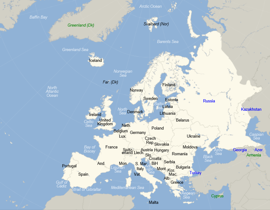
But some basic facts, for orientation. The 2013 population of Europe, shown in the following map, is estimated at just above 740 million persons. This makes Europe a little over 10 percent of total global population.

europe

The European Union (EU) includes 28 countries, as follows with their date of entry in parenthesis:

Austria (1995), Belgium (1952), Bulgaria (2007), Croatia (2013), Cyprus (2004), Czech Republic (2004), Denmark (1973), Estonia (2004), Finland (1995), France (1952), Germany (1952), Greece (1981), Hungary (2004), Ireland (1973), Italy (1952), Latvia (2004), Lithuania (2004), Luxembourg (1952), Malta (2004), Netherlands (1952), Poland (2004), Portugal (1986), Romania (2007), Slovakia (2004), Slovenia (2004), Spain (1986), Sweden (1995), United Kingdom (1973).

The EU site states that –

The single or ‘internal’ market is the EU’s main economic engine, enabling most goods, services, money and people to move freely. Another key objective is to develop this huge resource to ensure that Europeans can draw the maximum benefit from it.

There also are governing bodies which are headquartered for the most part in Brussels and administrative structures.

The Eurozone consists of 18 European Union countries which have adopted the euro as their common currency. These countries includes Belgium, Germany, Estonia, Ireland, Greece, Spain, France, Italy, Cyprus, Latvia, Luxembourg, Malta, the Netherlands, Austria, Portugal, Slovenia, Slovakia and Finland.

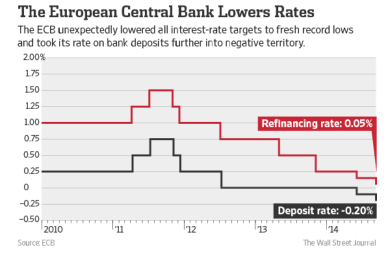
The European Central Bank (ECB) is located in Frankfurt, Germany and performs a number of central bank functions, but does not clearly state its mandate on its website, so far as I can discover. The ECB has a governing council comprised of representatives from Eurozone banking and finance circles.

Economic Significance of Europe

Something like 160 out of the Global 500 Corporations identified by Fortune magazine are headquartered in Europe – and, of course, tax slides are moving more and more US companies to nominally move their operations to Europe.

According to the International Monetary Fund World Economic Outlook (July 14, 2013 update), the Eurozone accounts for an estimated 17 percent of global output, while the European Union countries comprise an estimated 24 percent of global output. By comparison the US accounts for 23 percent of global output, where all these percents are measured in terms of output in current US dollar equivalents.

What is the Problem?

I began engaging with Europe and its economic setup professionally, some years ago. The European market is important to information technology (IT) companies. Europe was a focus for me in 2008 and through the so-called Great Recession, when sharp drops in output occurred on both sides of the Atlantic. Then, after 2009 for several years, the impact of the global downturn continued to be felt in Europe, especially in the Eurozone, where there was alarm about the possible breakup of the Eurozone, defaults on sovereign debt, and massive banking failure.

I have written dozens of pages on European economic issues for circulation in business contexts. It’s hard to distill all this into a more current perspective, but I think the Greek economist Yanis Varoufakis does a fairly good job.

Let me cite two posts – WHY IS EUROPE NOT ‘COMING TOGETHER’ IN RESPONSE TO THE EURO CRISIS? and MODEST PROPOSAL.

The first quote highlights the problems (and lure) of a common currency to a weaker economy, such as Greece.

Right from the beginning, the original signatories of the Treaty of Rome, the founding members of the European Economic Community, constituted an asymmetrical free trade zone….

To see the significance of this asymmetry, take as an example two countries, Germany and Greece today (or Italy back in the 1950s). Germany, features large oligopolistic manufacturing sectors that produce high-end consumption as well as capital goods, with significant economies of scale and large excess capacity which makes it hard for foreign competitors to enter its markets. The other, Greece for instance, produces next to no capital goods, is populated by a myriad tiny firms with low price-cost margins, and its industry has no capacity to deter competitors from entering.

By definition, a country like Germany can simply not generate enough domestic demand to absorb the products its capital intensive industry can produce and must, thus, export them to the country with the lower capital intensity that cannot produce these goods competitively. This causes a chronic trade surplus in Germany and a chronic trade deficit in Greece.

If the exchange rate is flexible, it will inevitably adjust, constantly devaluing the currency of the country with the lower price-cost margins and revaluing that of the more capital-intensive economy. But this is a problem for the elites of both nations. Germany’s industry is hampered by uncertainty regarding how many DMs it will receive for a BMW produced today and destined to be sold in Greece in, say, ten months. Similarly, the Greek elites are worried by the devaluation of the drachma because, every time the drachma devalues, their lovely homes in the Northern Suburbs of Athens, or indeed their yachts and other assets, lose value relative to similar assets in London and Paris (which is where they like to spend their excess cash). Additionally, Greek workers despise devaluation because it eats into every small pay rise they manage to extract from their employers. This explains the great lure of a common currency to Greeks and to Germans, to capitalists and labourers alike. It is why, despite the obvious pitfalls of the euro, whole nations are drawn to it like moths to the flame.

So there is a problem within the Eurozone of “recycling trade surpluses” basically from Germany and the stronger members to peripheral countries such as Greece, Portugal, Ireland, and even Spain – where Italy is almost a special, but very concerning case.

The next quote is from a section in MODEST PROPOSAL called “The Nature of the Eurozone Crisis.” It is is about as succinct an overview of the problem as I know of – without being excessively ideological.

The Eurozone crisis is unfolding on four interrelated domains.

Banking crisis: There is a common global banking crisis, which was sparked off mainly by the catastrophe in American finance. But the Eurozone has proved uniquely unable to cope with the disaster, and this is a problem of structure and governance. The Eurozone features a central bank with no government, and national governments with no supportive central bank, arrayed against a global network of mega-banks they cannot possibly supervise. Europe’s response has been to propose a full Banking Union – a bold measure in principle but one that threatens both delay and diversion from actions that are needed immediately.

Debt crisis: The credit crunch of 2008 revealed the Eurozone’s principle of perfectly separable public debts to be unworkable. Forced to create a bailout fund that did not violate the no-bailout clauses of the ECB charter and Lisbon Treaty, Europe created the temporary European Financial Stability Facility (EFSF) and then the permanent European Stability Mechanism (ESM). The creation of these new institutions met the immediate funding needs of several member-states, but retained the flawed principle of separable public debts and so could not contain the crisis. One sovereign state, Cyprus, has now de facto gone bankrupt, imposing capital controls even while remaining inside the euro.

During the summer of 2012, the ECB came up with another approach: the Outright Monetary Transactions’ Programme (OMT). OMT succeeded in calming the bond markets for a while. But it too fails as a solution to the crisis, because it is based on a threat against bond markets that cannot remain credible over time.

And while it puts the public debt crisis on hold, it fails to reverse it; ECB bond purchases cannot restore the lending power of failed markets or the borrowing power of failing governments.

Investment crisis: Lack of investment in Europe threatens its living standards and its international competitiveness. As Germany alone ran large surpluses after 2000, the resulting trade imbalances ensured that when crisis hit in 2008, the deficit zones would collapse. And the burden of adjustment fell exactly on the deficit zones, which could not bear it. Nor could it be offset by devaluation or new public spending, so the scene was set for disinvestment in the regions that needed investment the most.

Thus, Europe ended up with both low total investment and an even more uneven distribution of that investment between its surplus and deficit regions.

Social crisis: Three years of harsh austerity have taken their toll on Europe’s peoples. From Athens to Dublin and from Lisbon to Eastern Germany, millions of Europeans have lost access to basic goods and dignity. Unemployment is rampant. Homelessness and hunger are rising. Pensions have been cut; taxes on necessities meanwhile continue to rise. For the first time in two generations, Europeans are questioning the European project, while nationalism, and even Nazi parties, are gaining strength.

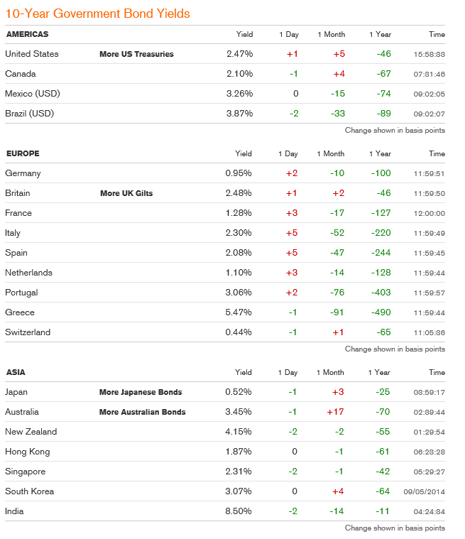
This is from a white paper jointly authored by Yanis Varoufakis, Stuart Holland and James K. Galbraith which offers a rationale and proposal for a European “New Deal.” In other words, take advantage of the record low global interest rates and build infrastructure.

The passage covers quite a bit of ground without appearing to be comprehensive. However, it will be be a good guide to check, I think, if a significant downturn unfolds in the next few quarters. Some of the nuances will come to life, as flaws in original band-aid solutions get painfully uncovered.

Now there is no avoiding some type of ideological or political stance in commenting on these issues, but the future is the real question. What will happen if a recession takes hold in the next few quarters?

More on European Banks

European banks have been significantly under-capitalized, as the following graphic from before the Great Recession highlights.

bankleverage

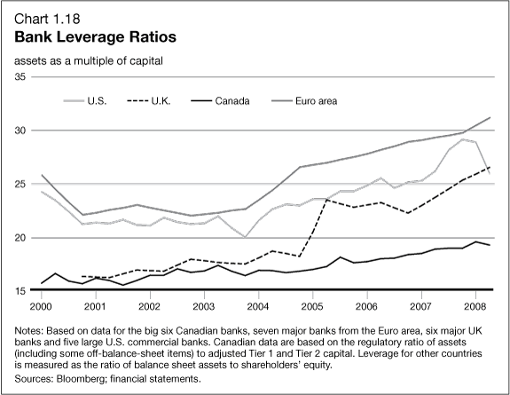
Another round of stress tests are underway by the ECB, and, according to the Wall Street Journal, will be shared with banks in coming weeks. Significant recapitalization of European banks, often through stock issues, has taken place. Things have moved forward from the point at which, last year, the US Federal Deposit Insurance Corporation (FDIC) Vice Chairman called Deutsche Banks capitalization ratios “horrible,” “horribly undercapitalized” and with “no margin of error.”

Bottom LIne

If a recession unfolds in the next few quarters, it is likely to significantly impact the European economy, opening up old wounds, so to speak, wounds covered with band-aid solutions. I know I have not proven this assertion in this post, but it is a message I want to convey.

The banking sector is probably where the problems will first flare up, since banks have significant holdings of sovereign debt from EU states that already are on the ropes – like Greece, Spain, Portugal, and Italy. There also appears to be some evidence of froth in some housing markets, with record low interest rates and the special conditions in the UK.

Hopefully, the global economy can side-step this current wobble from the first quarter 2014 and maybe even further in some quarters, and somehow sustain positive or at least zero growth for a few years.

Otherwise, this looks like a house of cards.

Negative Nominal Interest Rates – the European Central Bank Experiment

Larry Summers, former US Treasury Secretary and, earlier, President of Harvard delivered a curious speech at an IMF Economic Forum last year. After nice words about Stanley Fischer, currently Vice Chair of the Fed, Summers entertains the notion of negative interest rates to combat secular stagnation and restore balance between aggregate demand and supply at something like full employment.

Fast forward to June 2014, when the European Central Bank (ECB) pushes the interest rate on deposits European banks hold in the ECB into negative territory. And on September 4, the ECB drops the deposit rates further to -0.2 percent, also reducing a refinancing rate to virtually zero.

ECBnegint

The ECB discusses this on its website – Why Has the ECB Introduced a Negative interest Rate. After highlighting the ECB mandate to ensure price stability by aiming for an inflation rate of below but close to 2% over the medium term, the website observes euro area inflation is expected to remain considerably below 2% for a prolonged period.

This provides a rationale for lower interest rates, of which there are principally three under ECB control – a marginal lending facility for overnight lending to banks, the main refinancing operations and the deposit facility.

Note that the main refinancing rate is the rate at which banks can regularly borrow from the ECB while the deposit rate is the rate banks receive for funds parked at the central bank.

The ECB is adjusting interest rates under their control across the board, as suggested by the chart, but worries that to maintain a functioning money market in which commercial banks lend to each other, these rates cannot be too close to each other.

So, bottom line, the deposit rate was lowered to − 0.10 % in June to maintain this corridor, and then further as the refinancing rate was dropped to -.05 percent.

The hope is that lower refinancing rates will mean lower rates for customers for bank loans, while negative deposit rates will act as a disincentive for banks to simply park excess reserves in the ECB.

Nominal Versus Real Interest Rates and Bond Yields

If you want to prep for, say, negative yields on two year Irish bonds, or issuance of various European bonds with negative yield, as well as the negative yields of a variety of US securities in recent years, after inflation, check out How Low Can You Go? Negative Interest Rates and Investors’ Flight to Safety.

An asset can generate a negative yield, on a conventional, rather than catastrophic basis, in a nominal or real, which is to say, inflation-adjusted, sense.

Some examples of negative real interest rates of yields –

The yield to maturity on the 5-year Treasury note has been below 2 percent since July 2010, and the yield to maturity on the 10-year Treasury note has been below 2 percent since May 2012. Yet, looking forward, the Federal Open Market Committee in January 2012 announced an inflation target of 2 percent—implying an anticipated negative real yield over the life of the securities. Investors, facing uncertainty, appear willing to pay the U.S. government—when measured in real, ex post inflation-adjusted dollars—for the privilege of owning Treasury securities.

And the current government bond yield situation, from Bloomberg, shows important instances of negative yields, notably Germany and Japan – two of the largest global economies. Click to enlarge.

bondyields

Where the ECB Goes From Here

Mario Draghi, ECB head, gave a speech clearly stating monetary policy is not enough, at the recent Jackson Hole conference of central bankers. After this, the financial press was abuzz with the idea Draghi is moving toward the Japanese leader Abe’s formulation in which there are three weapons or arrows in the Japanese formulation– monetary policy, fiscal policy and structural reforms.

The problem, in the case of the Eurozone, is achieving political consensus for fiscal policies such as backing bonds for badly needed infrastructure development. German opposition seems to be sustained and powerful.

Because of the “political economy” factors , currency and banking problems in the Eurozone are probably more complicated and puzzling than many business executives and managers, looking for a take on the situation, would prefer.

A Thought Experiment

Before diving into this conceptually hazardous topic, though, I’d like to pose a puzzle for readers.

Can banks realistically “charge” negative interest rates to commercial customers?

I seem to have cooked up a spreadsheet where such loans could pay a rate of positive real return to banks, if the rate of deflation can be projected.  In one variant, the bank collects a lending fee at the outset and then the interest rate for installments is negative.

The “save” for banks is that future deflation could inflate the real value of declining nominal installment payments, creating a present value of this stream of payments which is greater than the simple sum of such payments.

I’m not ready for primetime television with this, but it seems such a world encapsulates a very dour view of the future – one that may not be too far from the actual situation in Europe and Japan.

Money black hole at top from Conservative Read

Something is Happening in Europe

Something is going on in Europe.

Take a look at this chart of the euro/dollar exchange rate, and how some event triggered a step down mid week of last week (from xe.com).

euroexchange

The event in question was a press conference by Mario Draghi (See the Wall Street Journal real time blog on this event at Mario Draghi Delivers Fresh ECB Plan — Recap).

The European Central Bank under Draghi is moving into exotic territory – trying negative interest rates on bank deposits and toying with variants of Quantitative Easing (QE) involving ABS – asset backed securities.

All because the basic numbers for major European economies, including notably Germany and France (as well as long-time problem countries such as Spain), are not good. Growth has stalled or is reversing, bank lending is falling, and deflation stalks the European markets.

Europe – which, of course, is sectored into the countries inside and outside the currency union, countries in the common market, and countries in none of the above – accounts for several hundred million persons and maybe 20-30 percent of global production.

So what happens there is significant.

Then there is the Ukraine crisis.

Zerohedge ran this graphic recently showing the dependence of European countries on gas from Russia.

eurdependence

The US-led program of imposing sanctions on Russia – key individuals, companies, banks perhaps – flies in the face of the physical dependence of Germany, for example, on Russian gas.

On the other hand, there is lots of history here on all sides, including, notably, the countries formerly in the USSR in eastern Europe, who no doubt fear the increasingly nationalistic or militant stance shown by Russia currently in, for example, re-acquiring Crimea.

As Chancellor Merkel has stressed, this is an area for diplomacy and negotiation – although there are other voices and forces ready to rush more weapons and even troops to the region of conflict.

Finally, as I have been stressing from time to time, there is an emerging demographic reality which many European nations have to confront.

Edward Hugh has several salient posts on possibly overlooked impacts of aging on the various macroeconomies involved.

There also is the vote on Scotland coming up in the United Kingdom (what we may, if the “yes” votes carry, need to start calling “the British Isles.”)

I’d like to keep current with the signals coming from Europe in a few blogs upcoming – to see, for example, whether swing events in the next six months to a year could originate there.

Mid-Year Economic Projections and Some Fireworks

Greetings and Happy Fourth of July! Always one of my favorite holidays.

Practically every American kid loves the Fourth, because there are fireworks. Of course, back in the day, we had cherry bombs and really big firecrackers. Lots of thumbs and fingers were blown off. But it’s still fun for kids, and safer no doubt.

Before that, here are two mid-year forecasts from Goldman Sachs’ Chief Economist Jan Hatzius and an equity outlook from Wells Fargo Bank.

Jan Hatzius Goldman Sachs – mid-year forecast (June 12) 

And Wells Fargo (June 23rd). 

Both these, unfortunately, did not have the information about the additional write-down of the 1st quarter real GDP that came out June 25, so we will be looking for futher updates.

Meanwhile, some fireworks.

First, Happy Fourth from the US Navy. 

And some ordinary fireworks from the National Mall, US Capitol, 2012. 

Distributions of Stock Returns and Other Asset Prices

This is a kind of wrap-up discussion of probability distributions and daily stock returns.

When I did autoregressive models for daily stock returns, I kept getting this odd, pointy, sharp-peaked distribution of residuals with heavy tails. Recent posts have been about fitting a Laplace distribution to such data.

I have recently been working with the first differences of the logarithm of daily closing prices – an entity the quantitative finance literature frequently calls “daily returns.”

It turns out many researchers have analyzed the distribution of stock returns, finding fundamental similarities in the resulting distributions. There are also similarities for many stocks in many international markets in the distribution of trading volumes and the number of trades. These similarities exist at a range of frequencies – over a few minutes, over trading days, and longer periods.

The paradigmatic distribution of returns looks like this:

NASDAQDR

This is based on closing prices of the NASDAQ 100 from October 1985 to the present.

There also are power laws that can be extracted from the probabilities that the absolute value of returns will exceed a certain amount.

For example, again with daily returns from the NASDAQ 100, we get an exponential distribution if we plot these probabilities of exceedance. This curve can be fit by a relationship ~x where θ is between 2.7 and 3.7, depending on where you start the estimation from the top or largest probabilities.

NASDAQABSDR

These magnitudes of the exponent are significant, because they seem to rule out whole classes, such as Levy stable distributions, which require θ < 2.

Also, let me tell you why I am not “extracting the autoregressive components” here. There are probably nonlinear lag effects in these stock price data. So my linear autoregressive equations probably cannot extract all the time dependence that exist in the data. For that reason, and also because it seems pro forma in quantitative finance, my efforts have turned to analyzing what you might call the raw daily returns calculated with price data and suitable transformations.

Levy Stable Distributions

At the turn of the century, Mandelbrot, then Sterling Professor of Mathematics at Yale, wrote an introductory piece for a new journal called Quantitative Finance called Scaling in financial prices: I. Tails and dependence. In that piece, which is strangely convoluted by my lights, Mandelbrot discusses how he began working with Levy-stable distributions in the 1960’s to model the heavy tails of various stock and commodity price returns.

The terminology is a challenge, since there appear to be various ways of discussing so-called stable distributions, which are distributions which yield other distributions of the same type under operations like summing random variables, or taking their ratios.

The Quantitative Finance section of Stack Exchange has a useful Q&A on Levy-stable distributions in this context.

Answers refer readers to Nolan’s 2005 paper Modeling Financial Data With Stable Distributions which tells us that the class of all distributions that are sum-stable is described by four parameters. The distributions controlled by these parameters, however, are generally not accessible as closed algebraic expressions, but must be traced out numerically by computer computations.

Nolan gives several applications, for example, to currency data, illustrated with the following graphs.

Nolan1

So, the characteristics of the Laplace distribution I find so compelling are replicated to an extent by the Levy-stable distributions.

While Levy-stable distributions continue to be the focus of research in some areas of quantitative finance – risk assessment, for instance – it’s probably true that applications to stock returns are less popular lately. There are two reasons in particular. First, Levy stable distributions apparently have infinite variance, and as Cont writes, there is conclusive evidence that stock prices have finite second moments. Secondly, Levy stable distributions imply power laws for the probability of exceedance of a given level of absolute value of returns, but unfortunately these power laws have an exponent less than 2.

Neither of these “facts” need prove conclusive, though. Various truncated versions of Levy stable distributions have been used in applications like estimating Value at Risk (VAR).

Nolan also maintains a webpage which addresses some of these issues, and provides tools to apply Levy stable distributions.

Why Do These Regularities in Daily Returns and Other Price Data Exist?

If I were to recommend a short list of articles as “must-reads” in this field, Rama Cont’s 2001 survey in Quantitative Finance would be high on the list, as well as Gabraix et al’s 2003 paper on power laws in finance.

Cont provides a list of11 stylized facts regarding the distribution of stock returns.

1. Absence of autocorrelations: (linear) autocorrelations of asset returns are often insignificant, except for very small intraday time scales (

20 minutes) for which microstructure effects come into play.

2. Heavy tails: the (unconditional) distribution of returns seems to display a power-law or Pareto-like tail, with a tail index which is finite, higher than two and less than five for most data sets studied. In particular this excludes stable laws with infinite variance and the normal distribution. However the precise form of the tails is difficult to determine.

3. Gain/loss asymmetry: one observes large drawdowns in stock prices and stock index values but not equally large upward movements.

4. Aggregational Gaussianity: as one increases the time scale t over which returns are calculated, their distribution looks more and more like a normal distribution. In particular, the shape of the distribution is not the same at different time scales.

5. Intermittency: returns display, at any time scale, a high degree of variability. This is quantified by the presence of irregular bursts in time series of a wide variety of volatility estimators.

6. Volatility clustering: different measures of volatility display a positive autocorrelation over several days, which quantifies the fact that high-volatility events tend to cluster in time.

7. Conditional heavy tails: even after correcting returns for volatility clustering (e.g. via GARCH-type models), the residual time series still exhibit heavy tails. However, the tails are less heavy than in the unconditional distribution of returns.

8. Slow decay of autocorrelation in absolute returns: the autocorrelation function of absolute returns decays slowly as a function of the time lag, roughly as a power law with an exponent β ∈ [0.2, 0.4]. This is sometimes interpreted as a sign of long-range dependence.

9. Leverage effect: most measures of volatility of an asset are negatively correlated with the returns of that asset.

10. Volume/volatility correlation: trading volume is correlated with all measures of volatility.

11. Asymmetry in time scales: coarse-grained measures of volatility predict fine-scale volatility better than the other way round.

There’s a huge amount here, and it’s very plainly and well stated.

But then why?

Gabraix et al address this question, in a short paper published in Nature.

Insights into the dynamics of a complex system are often gained by focusing on large fluctuations. For the financial system, huge databases now exist that facilitate the analysis of large fluctuations and the characterization of their statistical behavior. Power laws appear to describe histograms of relevant financial fluctuations, such as fluctuations in stock price, trading volume and the number of trades. Surprisingly, the exponents that characterize these power laws are similar for different types and sizes of markets, for different market trends and even for different countries suggesting that a generic theoretical basis may underlie these phenomena. Here we propose a model, based on a plausible set of assumptions, which provides an explanation for these empirical power laws. Our model is based on the hypothesis that large movements in stock market activity arise from the trades of large participants. Starting from an empirical characterization of the size distribution of those large market participants (mutual funds), we show that the power laws observed in financial data arise when the trading behaviour is performed in an optimal way. Our model additionally explains certain striking empirical regularities that describe the relationship between large fluctuations in prices, trading volume and the number of trades.

The kernel of this paper in Nature is as follows:

powerlaws

Thus, Gabraix links the distribution of purchases in stock and commodity markets with the resulting distribution of daily returns.

I like this hypothesis and see ways it connects with the Laplace distribution and its variants. Probably, I will write more about this in a later post.

Microsoft Stock Prices and the Laplace Distribution

The history of science, like the history of all human ideas, is a history of irresponsible dreams, of obstinacy, and of error. But science is one of the very few human activities perhaps the only one in which errors are systematically criticized and fairly often, in time, corrected. This is why we can say that, in science, we often learn from our mistakes, and why we can speak clearly and sensibly about making progress there. — Karl Popper, Conjectures and Refutations

Microsoft daily stock prices and oil futures seem to fall in the same class of distributions as those for the S&P 500 and NASDAQ 100 – what I am calling the Laplace distribution.

This is contrary to the conventional wisdom. The whole thrust of Box-Jenkins time series modeling seems to be to arrive at Gaussian white noise. Most textbooks on econometrics prominently feature normally distributed error processes ~ N(0,σ).

Benoit Mandelbrot, of course, proposed alternatives as far back as the 1960’s, but still we find aggressive application of Gaussian assumptions in applied work – as for example in widespread use of the results of the Black-Scholes theorem or in computing value at risk in portfolios.

Basic Steps

I’m taking a simple approach.

First, I collect daily closing prices for a stock index, stock, or, as you will see, for commodity futures.

Then, I do one of two things: (a) I take the natural logarithms of the daily closing prices, or (b) I simply calculate first differences of the daily closing prices.

I did not favor option (b) initially, because I can show that the first differences, in every case I have looked at, are autocorrelated at various lags. In other words, these differences have an algorithmic structure, although this structure usually has weak explanatory power.

However, it is interesting that the first differences, again in every case I have looked at, are distributed according to one of these sharp-peaked or pointy distributions which are highly symmetric.

Take the daily closing prices of the stock of the Microsoft Corporation (MST), as an example.

Here is a graph of the daily closing prices.

MSFTgraph

And here is a histogram of the raw first differences of those closing prices over this period since 1990.

rawdifMSFT

Now in close reading of The Laplace Distribution and Generalizations I can see there are a range of possibilities in modeling distributions of the above type.

And here is another peaked, relatively symmetric distribution based on the residuals of an autoregressive equation calculated on the first differences of the logarithm of the daily closing prices. That’s a mouthful, but the idea is to extract at least some of the algorithmic component of the first differences.

MSFTregreshisto

That regression is as follows.

MSFTreg

Note the deep depth of the longest lags.

This type of regression, incidentally, makes money in out-of-sample backcasts, although possibly not enough to exceed trading costs unless the size of the trade is large. However, it’s possible that some advanced techniques, such as bagging and boosting, regression trees and random forecasts could enhance the profitability of trading strategies.

Well, a quick look at daily oil futures (CLQ4) from 2007 to the present.

oilfutures

Not quite as symmetric, but still profoundly not a Gaussian distribution.

The Difference It Makes

I’ve got to go back and read Mandelbrot carefully on his analysis of stock and commodity prices. It’s possible that these peaked distributions all fit in a broad class including the Laplace distribution.

But the basic issue here is that the characteristics of these distributions are substantially different than the Gaussian or normal probability distribution. This would affect maximum likelihood estimation of parameters in models, and therefore could affect regression coefficients.

Furthermore, the risk characteristics of assets whose prices have these distributions can be quite different.

And I think there is a moral here about the conventional wisdom and the durability of incorrect ideas.

Top pic is Karl Popper, the philosopher of science

The NASDAQ 100 Daily Returns and Laplace Distributed Errors

I once ran into Norman Mailer at the Museum of Modern Art in Manhattan. We were both looking at Picasso’s “Blue Boy” and, recognizing him, I started up some kind of conversation, and Mailer was quite civil about the whole thing.

I mention this because I always associate Mailer with his collection Advertisements for Myself.

And that segues – loosely – into my wish to let you know that, in fact, I developed a generalization of the law of demand for the situation in which a commodity is sold at a schedule of rates and fees, instead of a uniform price. That was in 1987, when I was still a struggling academic and beginning a career in business consulting.

OK, and that relates to a point I want to suggest here. And that is that minor players can have big ideas.

So I recognize an element of “hubris” in suggesting that the error process of S&P 500 daily returns – up to certain transformations – is described by a Laplace distribution.

What about other stock market indexes, then? This morning, I woke up and wondered whether the same thing is true for, say, the NASDAQ 100.

NASDAQ100

So I downloaded daily closing prices for the NASDAQ 100 from Yahoo Finance dating back to October 1, 1985. Then, I took the natural log of each of these closing prices. After that, I took trading day by trading day differences. So the series I am analyzing comes from the first differences of the natural log of the NASDAQ 100 daily closing prices.

Note that this series of first differences is sometimes cast into a histogram by itself – and this also frequently is a “pointy peaked” relatively symmetric distribution. You could motivate this graph with the idea that stock prices are a random walk. So if you take first differences, you get the random component that generates the random walk.

I am troubled, however, by the fact that this component has considerable structure in and of itself. So I undertake further analysis.

For example, the autocorrelation function of these first differences of the log of NASDAQ 100 daily closing prices looks like this.

NASDAQAC

Now if you calculate bivariate regressions on these first differences and their lagged values, many of them produce coefficient estimates with t-statistics that exceed the magic value of 2.

Just selecting these significant regressors from the first 47 lags produces this regression equation, I get this equation.

Regression

Now this regression is estimated over all 7200 observations from October 1 1984 to almost right now.

Graphing the residuals, I get the familiar pointy-peaked distribution that we saw with the S&P 500.

LaplaceNASDAQ100

Here is a fit of the Laplace distribution to this curve (Again using EasyFit).

EFLNQ

Here are the metrics for this fit and fits to a number of other probability distributions from this program.

EFtable

I have never seen as clear a linkage of returns from stock indexes and the Laplace distribution (maybe with a slight asymmetry – there are also asymmetric Laplace distributions).

One thing is for sure – the distribution above for the NASDAQ 100 data and the earlier distribution developed for the S&P 500 are not close to be normally distributed. Thus, in the table above that the normal distribution is number 12 on the list of possible candidates identified by EasyFit.

Note “Error” listed in the above table, is not the error function related to the normal distribution. Instead it is another exponential distribution with an absolute value in the exponent like the Laplace distribution. In fact, it looks like a transformation of the Laplace, but I need to do further investigation. In any case, it’s listed as number 2, even though the metrics show the same numbers.

The plot thickens.

Obviously, the next step is to investigate individual stocks with respect to Laplacian errors in this type of transformation.

Also, some people will be interested in whether the autoregressive relationship listed above makes money under the right trading rules. I will report further on that.

Anyway, thanks for your attention. If you have gotten this far – you believe numbers have power. Or you maybe are interested in finance and realize that indirect approaches may be the best shot at getting to something fundamental.

The Laplace Distribution and Financial Returns

Well, using EasyFit from Mathwave, I fit a Laplace distribution to the residuals of the regression on S&P daily returns I discussed yesterday.

Here is the result.

Laplacefit

This beats a normal distribution hands down. It also appears to beat the Matlab fit of a t distribution, but I have to run down more details on forms of the t-distribution to completely understand what is going on in the Matlab setup.

Note that EasyFit is available for a free 30-day trial download. It’s easy to use and provides metrics on goodness of fit to make comparisons between distributions.

There is a remarkable book online called The Laplace Distribution and Generalizations. If you have trouble downloading it from the site linked here, Google the title and find the download for a free PDF file.

This book, dating from 2001, runs to 458 pages, has a good introductory discussion, extensive mathematical explorations, as well as applications to engineering, physical science, and finance.

The French mathematical genius Pierre Simon Laplace proposed the distribution named after him as a first law of errors when he was 25, before his later discussions of the normal distribution.

The normal probability distribution, of course, “took over” – in part because of its convenient mathematical properties and also, probably, because a lot of ordinary phenomena are linked with Gaussian processes.

John Maynard Keynes, the English economist, wrote an early monograph (Keynes, J.M. (1911). The principal averages and the laws of error which lead to them, J. Roy. Statist. Soc. 74, New Series, 322-331) which substantially focuses on the Laplace distribution, highlighting the importance it gives to the median, rather than average, of sample errors.

The question I’ve struggled with is “why should stock market trading, stock prices, stock indexes lead, after logarithmic transformation and first differencing to the Laplace distribution?”

Of course, the Laplace distribution can be generated as a difference of exponential distributions, or as combination of a number of distributions, as the following table from Kotz, Kozubowski, and Podgorski’s book shows.

Ltable

This is all very suggestive, but how can it be related to the process of trading?

Indeed, there are quite a number of questions which follow from this hypothesis – that daily trading activity is fundamentally related to a random component following a Laplace distribution.

What about regression, if the error process is not normally distributed? By following the standard rules on “statistical significance,” might we be led to disregard variables which are drivers for daily returns or accept bogus variables in predictive relationships?

Distributional issues are important, but too frequently disregarded.

I recall a blog discussion by a hedge fund trader lamenting excesses in the application of the Black-Scholes Theorem to options in 2007 and thereafter.

Possibly, the problem is as follows. The residuals of autoregressions on daily returns and their various related transformations tend to cluster right around zero, but have big outliers. This clustering creates false confidence, making traders vulnerable to swings or outliers that occur much more frequently than suggested by a normal or Gaussian error distribution.

The Distribution of Daily Stock Market Returns

I think it is about time for another dive into stock market forecasting. The US market is hitting new highs with the usual warnings of excess circulating around. And there are interesting developments in volatility.

To get things rolling, consider the following distribution of residuals from an autoregressive model on the difference in the natural logarithms of the S&P 500.

This is what I am calling “the distribution of daily stock market returns.” I’ll explain that further in a minute.

residualsLSPD

Now I’ve seen this distribution before, and once asked in a post, “what type of distribution is this?”

Now I think I have the answer – it’s a Laplace distribution, sometimes known as the double exponential distribution.

Since this might be important, let me explain the motivation and derivation of these residuals, and then consider some implications.

Derivation of the Residuals

First, why not just do a histogram of the first differences of daily returns to identify the underlying distribution? After all, people say movement of stock market indexes are a random walk.

OK, well you could do that, and the resulting distribution would also look “Laplacian” with a pointy peak and relative symmetry. However, I am bothered in developing this by the fact that these first differences show significant, even systematic, autocorrelation.

I’m influenced here by the idea that you always want to try to graph independent draws from a distribution to explore the type of distribution.

OK, now to details of my method.

The data are based on daily closing values for the S&P 500 index from December 4, 1989 to February 7, 2014.

I took the natural log of these closing values and then took first differences – subtracting the previous trading day’s closing value from the current day’s closing value. This means that these numbers encode the critical part of the daily returns, which are calculated as day-over-day percent changes. Thus, the difference of natural logs is in fact a ratio of the original numbers – what you might look at as the key part of the percent change from one trading day to the next.

So I generate a conventional series of first differences of the natural log of this nonstationary time series. This transforms the original nonstationary series to a  one that basically fluctuates around a level – essentially zero. Furthermore, the log transform tends to reduce the swings in the variability of the series, although significant variability remains.

1stdiflnsp

Removing Serial Correlation

The series graphed above exhibits first order serial correlation. It also exhibits second order serial correlation, or correlation between values at a lag of 2.

Based on the correlations for the first 24 lags, I put together this regression equation. Of course, the “x’s” refer to time dated first differences of the natural log of the S&P daily closing values.

reg1stdiflnsp

Note that most of the t-statistics pass our little test of significance (which I think is predicted to an extent on the error process belonging to certain distributions..but). The coefficient of determination or R2 is miniscule – at 0.017. This autoregressive equation thus explains only about 2 percent of the variation in this differenced log daily closing values series.

Now one of the things I plan to address is how, indeed, that faint predictive power can exert significant influence on earnings from stock trading, given trading rules.

But let me leave that whole area – how you make money with such a relationship – to a later discussion, since I’ve touched on this before.

Instead, let me just observe that if you subtract the predicted values from this regression from the actuals trading day by trading day, you get the data for the pointy, highly symmetric distribution of residuals.

Furthermore, these residuals do not exhibit first or second, or higher, autocorrelation, so far as I am able to determine.

This means we have separated out algorithmic components of this series from random components that are not serially correlated.

So you might jump to the conclusion that these residuals are then white noise, and I think many time series modelers have gotten to this point, simply assuming they are dealing with Gaussian white noise.

Nothing could be further from the truth, as the following Matlab fit of a normal distribution to some fairly crude bins for these numbers.

normfitLSPRes

A Student-t distribution does better, as the following chart shows.

TfitSPRes

But the t-distribution still misses the pointed peak.

The Laplace distribution is also called the double exponential, since it can be considered to be a composite of exponentials on the right and to the left of the mean – symmetric but mirror images of each other.

The following chart shows how this works over the positive residuals.

Exponposfit

Now, of course, there are likelihood ratios and those sorts of metrics, and I am busy putting together a comparison between the t-distribution fit and Laplace distribution fit.

There is a connection between the Laplace distribution and power laws, too, and I note considerable literature on this distribution in finance and commodities.

I think I have answered the question I put out some time back, though, and, of course, it raises other questions in its wake.