Tag Archives: forecasting controversy

Forecasting Controversy Swirling Around Computer Models and Forecasts

I am intrigued by Fabius Maximus’ We must rely on forecasts by computer models. Are they reliable?

This is a broad, but deeply relevant, question.

With the increasing prominence of science in public policy debates, the public’s beliefs about theories also have effects. Playing to this larger audience, scientists have developed an effective tool: computer models making bold forecasts about the distant future. Many fields have been affected, such as health care, ecology, astronomy, and climate science. With their conclusions amplified by activists, long-term forecasts have become a powerful lever to change pubic opinion.

It’s true. Large scale computer models are vulnerable to confirmation bias in their construction and selection – example being the testing of drugs. There are issues of measuring their reliability and — more fundamentally — validation (e.g., falsification).

Peer-review has proven quite inadequate to cope with these issues (which lie beyond the concerns about peer-review’s ability to cope with even standard research). A review or audit of a large model often requires over a man-years or more of work by a multidisciplinary team of experts, the kind of audit seldom done even on projects of great public concern.

Of course, FM is sort of famous, in my mind, for their critical attitude toward global warming and climate change.

And they don’t lose an opportunity to score points about climate science, citing the Georgia Institute of Technology scientist Judith Curry.

Dr. Curry is author of a recent WSJ piece The Global Warming Statistical Meltdown

At the recent United Nations Climate Summit, Secretary-General Ban Ki-moon warned that “Without significant cuts in emissions by all countries, and in key sectors, the window of opportunity to stay within less than 2 degrees [of warming] will soon close forever.” Actually, this window of opportunity may remain open for quite some time. A growing body of evidence suggests that the climate is less sensitive to increases in carbon-dioxide emissions than policy makers generally assume—and that the need for reductions in such emissions is less urgent.

A key issue in this furious and emotionally-charged debate is discussed in my September blogpost CO2 Concentrations Spiral Up, Global Temperature Stabilizes – Was Gibst?

..carbon dioxide (CO2) concentrations continue to skyrocket, while global temperature has stabilized since around 2000.

The scientific consensus (excluding Professor Curry and the climate change denial community) is that the oceans currently are absorbing the excess heat, but this cannot continue forever.

If my memory serves me (and I don’t have time this morning to run down the link), backtesting the Global Climate Models (GCM) in a recent IPCC methodology publication basically crashed and burned – but the authors blithely moved on to re-iterate the “consensus.”

At the same time, the real science behind climate change – the ice cores for example retrieved from glacial and snow and ice deposits of long tenure – do show abrupt change may be possible. Within a decade or two, for example, there might be regime shifts in global climate.

I am not going to draw conclusions at this point, wishing to carry on this thread with some discussion of macroeconomic models and forecasting.

But I leave you today with my favorite viewing of Blalog’s “Chasing Ice.”

Forecasting Controversy – the Polar Vortex

Three short, amusing videos to watch while keeping warm as the snow falls in Las Vegas and most other places are plunged into subzero weather.

The Polar Vortex Explained in 2 Minutes from the White House.

This video clip, originally distributed through the Office of Science and Technology Policy, kicked off the controversy.

Rush Limbaugh Response

Rush Limbaugh, always a reliable source on science and general systems theory, says the polar vortex was invented by liberal conspirators to scare folks.

Limbaugh is Full of Hot Air

Weatherman Al Roker fired back at Limbaugh’s ‘Polar Vortex’ Conspiracy, showing a page from his meteorology textbook from way back when, defining the term,”polar vortex.”

But can the Polar Vortex – recognized as a real weather phenomenon for decades – be forecast and is it related to climate change?

Well, this year there was an interesting split between weather forecasting services. As an article reacting to the October 16 release of the NWS Long Range Forecast notes .. the commercial forecasters are telling us to brace for the return of the Arctic air in the U.S. while the federal forecasters have countered by saying another wavy vortex dipping far south is “unlikely.”

Thus, we had NOAA: Another warm winter likely for western U.S., South may see colder weather           .

Well, the National Weather Service and its Canadian counterpart missed the big cold snap in November and the current incursion of artic air to lower lattitudes, due to shifting of the polar vortex.

Accuweather and the Weather Channel, on the other hand, scored big on their forecasts.

At the same time, Internet studies do not show that Accuweather has any leg up in long range forecasting –  snow in New York, for example – beyond a few days from the release of the forecast.

Also, the scientific basis for linking climate change and these polar vortex events is tenuous, or at least multi-factor.

Thus, a recent article in Nature – Weakening of the stratospheric polar vortex by Arctic sea-ice loss – concludes [footnote numbers removed] –

Through a combination of observation-based data analysis and climate model experiments, we provide corroborative evidence for the notion that Arctic sea-ice loss over the B–K seas plays an important role in weakening the stratospheric polar vortex. Regional sea-ice reductions over the B–K seas cause not only in situ surface warming but also significant upper-level responses that exhibit positive geopotential height anomalies over Eastern Europe and negative anomalies from East Asia to the Eastern Pacific along the wave-guide of the tropospheric westerly jet. This anomaly pattern projects heavily into the climatological wave, intensifying the vertical propagation of planetary-scale wave into the stratosphere and, in turn, weakening the stratospheric polar vortex. Therefore, planetary-scale wave generation by sea-ice losses and its upward propagation during early winter months underline the link between surface climate variability and polar stratospheric variability.

The weakened stratospheric polar vortex is often followed by a negative phase of the AO at the surface, favoring cold surface temperatures across Northern Hemisphere continents during the late winter months (Supplementary Fig. 1). Several physical mechanisms for this downward coupling have been proposed. They include the balanced response of the troposphere to stratospheric potential vorticity anomalies and wave-driven changes in the meridional circulation. It is also suggested that the tropospheric response involves changes in the synoptic eddies. However, it has been difficult to isolate the key process, and the detailed nonlinear processes involved are still under investigation21

As a final remark, we note that Arctic sea-ice loss represents only one of the possible factors that can affect the stratospheric polar vortex. Other factors reported in previous works include Eurasian snow cover, the Quasi Biannual Oscillation, the El-Nino and Southern Oscillation and solar activity.

I think it’s probably possible to show – through psychological and historical studies – that human decision-making over risky alternatives is most likely to fail with respect to (a) collective choices over (b) complex outcomes where target events have relatively low probability, although possibly huge costs. This makes the climate change issue and responding appropriately to it hugely difficult.

Top image from Medical Daily

Forecasting Controversies – Impacts of QE

Where there is smoke, there is fire, and other similar adages are suggested by an arcane statistical controversy over quantitative easing (QE) by the US Federal Reserve Bank.

Some say this Fed policy, estimated to have involved $3.7 trillion dollars in asset purchases, has been a bust, a huge waste of money, a give-away program to speculators, but of no real consequence to Main Street.

Others credit QE as the main force behind lower long term interest rates, which have supported US housing markets.

Into the fray jump two elite econometricians – Johnathan Wright of Johns Hopkins and Christopher Neeley, Vice President of the St. Louis Federal Reserve Bank.

The controversy provides an ersatz primer in estimation and forecasting issues with VAR’s (vector autoregressions). I’m not going to draw out all the nuances, but highlight the main features of the argument.

The Effect of QE Announcements From the Fed Are Transitory – Lasting Maybe Two or Three Months

Basically, there is the VAR (vector autoregression) analysis of Johnathan Wright of Johns Hopkins Univeristy, which finds that  –

..stimulative monetary policy shocks lower Treasury and corporate bond yields, but the effects die o¤ fairly fast, with an estimated half-life of about two months.

This is in a paper What does Monetary Policy do to Long-Term Interest Rates at the Zero Lower Bound? made available in PDF format dated May 2012.

More specifically, Wright finds that

Over the period since November 2008, I estimate that monetary policy shocks have a significant effect on ten-year yields and long-maturity corporate bond yields that wear o¤ over the next few months. The effect on two-year Treasury yields is very small. The initial effect on corporate bond yields is a bit more than half as large as the effect on ten-year Treasury yields. This finding is important as it shows that the news about purchases of Treasury securities had effects that were not limited to the Treasury yield curve. That is, the monetary policy shocks not only impacted Treasury rates, but were also transmitted to private yields which have a more direct bearing on economic activity. There is slight evidence of a rotation in breakeven rates from Treasury Inflation Protected Securities (TIPS), with short-term breakevens rising and long-term forward breakevens falling.

Not So, Says A Federal Reserve Vice-President

Christopher Neeley at the St. Louis Federal Reserve argues Wright’s VAR system is unstable and has poor performance in out-of-sample predictions. Hence, Wright’s conclusions cannot be accepted, and, furthermore, that there are good reasons to believe that QE has had longer term impacts than a couple of months, although these become more uncertain at longer horizons.

ChristopherNeely

Neeley’s retort is in a Federal Reserve working paper How Persistent are Monetary Policy Effects at the Zero Lower Bound?

A key passage is the following:

Specifically, although Wright’s VAR forecasts well in sample, it forecasts very poorly out-of-sample and fails structural stability tests. The instability of the VAR coefficients imply that any conclusions about the persistence of shocks are unreliable. In contrast, a naïve, no-change model out-predicts the unrestricted VAR coefficients. This suggests that a high degree of persistence is more plausible than the transience implied by Wright’s VAR. In addition to showing that the VAR system is unstable, this paper argues that transient policy effects are inconsistent with standard thinking about risk-aversion and efficient markets. That is, the transient effects estimated by Wright would create an opportunity for risk-adjusted  expected returns that greatly exceed values that are consistent with plausible risk aversion. Restricted VAR models that are consistent with reasonable risk aversion and rational asset pricing, however, forecast better than unrestricted VAR models and imply a more plausible structure. Even these restricted models, however, do not outperform naïve models OOS. Thus, the evidence supports the view that unconventional monetary policy shocks probably have fairly persistent effects on long yields but we cannot tell exactly how persistent and our uncertainty about the effects of shocks grows with the forecast horizon.

And, it’s telling, probably, that Neeley attempts to replicate Wright’s estimation of a VAR with the same data, checking the parameters, and then conducting additional tests to show that this model cannot be trusted – it’s unstable.

Pretty serious stuff.

Neeley gets some mileage out of research he conducted at the end of the 1990’s in Predictability in International Asset Returns: A Re-examination where he again called into question the longer term forecasting capability of VAR models, given their instabilities.

What is a VAR model?

We really can’t just highlight this controversy without saying a few words about VAR models.

A simple autoregressive relationship for a time series yt can be written as

yt = a1yt-1+..+anyt-n + et

Now if we have other variables (wt, zt..) and we write yt and all these other variables as equations in which the current values of these variables are functions of lagged values of all the variables.

The matrix notation is somewhat hairy, but that is a VAR. It is a system of autoregressive equations, where each variable is expressed as a linear sum of lagged terms of all the other variables.

One of the consequences of setting up a VAR is there are lots of parameters to estimate. So if p lags are important for each of three variables, each equation contains 3p parameters to estimate, so altogether you need to estimate 9p parameters – unless it is reasonable to impose certain restrictions.

Another implication is that there can be reduced form expressions for each of the variables – written only in terms of their own lagged values. This, in turn, suggests construction of impulse-response functions to see how effects propagate down the line.

Additionally, there is a whole history of Bayesian VAR’s, especially associated with the Minneapolis Federal Reserve and the University of Minnesota.

My impression is that, ultimately, VAR’s were big in the 1990’s, but did not live up to their expectations, in terms of macroeconomic forecasting. They gave way after 2000 to the Stock and Watson type of factor models. More variables could be encompassed in factor models than VAR’s, for one thing. Also, factor models often beat the naïve benchmark, while VAR’s frequently did not, at least out-of-sample.

The Naïve Benchmark

The naïve benchmark is a martingale, which often boils down to a simple random walk. The best forecast for the next period value of a martingale is the current period value.

This is the benchmark which Neeley shows the VAR model does not beat, generally speaking, in out-of-sample applications.

Naive

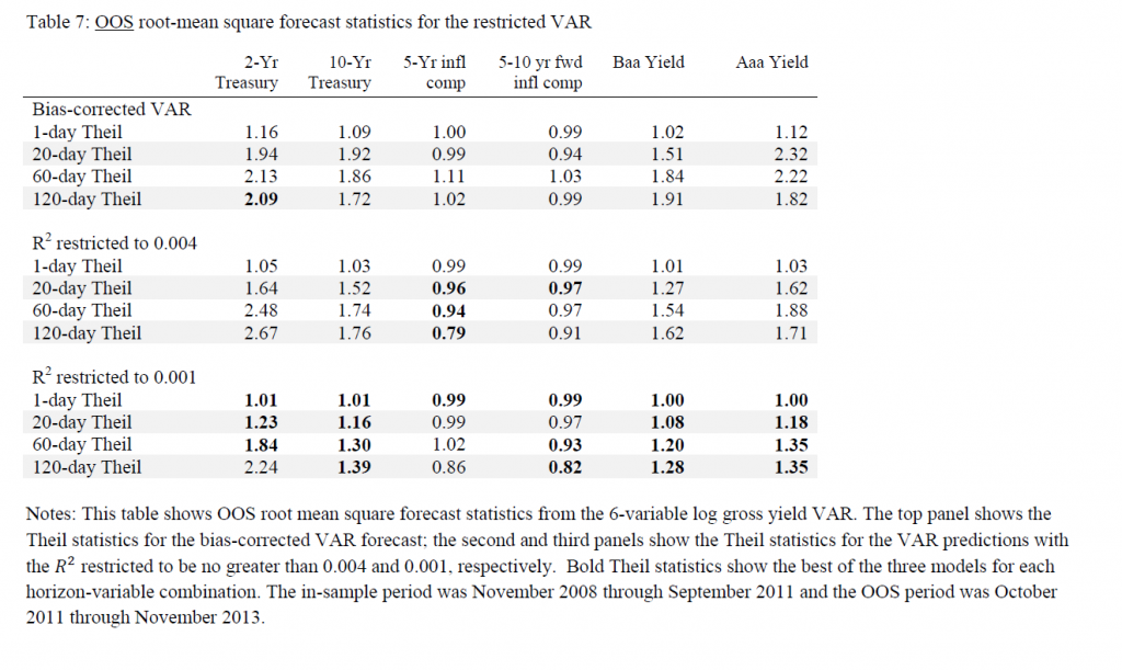
When the ratio is 1 or greater, this means that the mean square forecast error of the VAR is greater than the benchmark model.

Reflections

There are many fascinating details of these papers I am not highlighting. As an old Republican Congressman once said, “a billion here and a billion there, and pretty soon you are spending real money.”

So the defense of QE in this instance boils down to invalidating an analysis which suggests the impacts of QE are transitory, lasting a few months.

There is no proof, however, that QE has imparted lasting impacts on long term interest rates developed in this relatively recent research.