Tag Archives: gold price forecasts

Chinese economy, financial forecasting, stock market forecasts, technology forecasting

Links – Beginning of the Holiday Season

December 14, 2014 Clive Jones

Economy and Trade

Asia and Global Production Networks—Implications for Trade, Incomes and Economic Vulnerability Important new book –

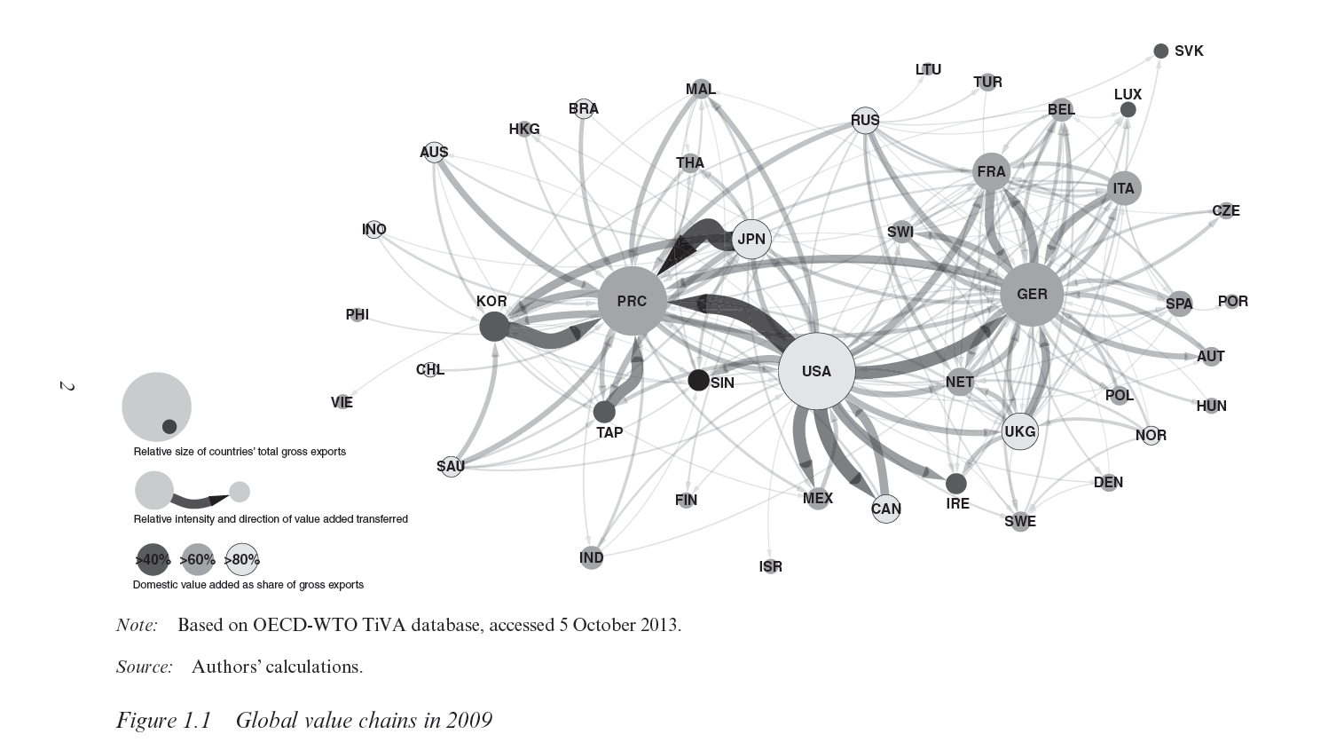
The publication has two broad themes. The first is national economies’ heightened exposure to adverse shocks (natural disasters, political disputes, recessions) elsewhere in the world as a result of greater integration and interdependence. The second theme is focused on the evolution of global value chains at the firm level and how this will affect competitiveness in Asia. It also traces the past and future development of production sharing in Asia.

Chapter 1 features the following dynamite graphic – (click to enlarge)

The Return of Currency Wars

Nouriel Roubini –

Central banks in China, South Korea, Taiwan, Singapore, and Thailand, fearful of losing competitiveness relative to Japan, are easing their own monetary policies – or will soon ease more. The European Central Bank and the central banks of Switzerland, Sweden, Norway, and a few Central European countries are likely to embrace quantitative easing or use other unconventional policies to prevent their currencies from appreciating.

All of this will lead to a strengthening of the US dollar, as growth in the United States is picking up and the Federal Reserve has signaled that it will begin raising interest rates next year. But, if global growth remains weak and the dollar becomes too strong, even the Fed may decide to raise interest rates later and more slowly to avoid excessive dollar appreciation.

The cause of the latest currency turmoil is clear: In an environment of private and public deleveraging from high debts, monetary policy has become the only available tool to boost demand and growth. Fiscal austerity has exacerbated the impact of deleveraging by exerting a direct and indirect drag on growth. Lower public spending reduces aggregate demand, while declining transfers and higher taxes reduce disposable income and thus private consumption.

Financial Markets

The 15 Most Valuable Startups in the World

Uber is among the top, raising $2.5 billion in direct investment funds since 2009. Airbnb, Dropbox, and many others.

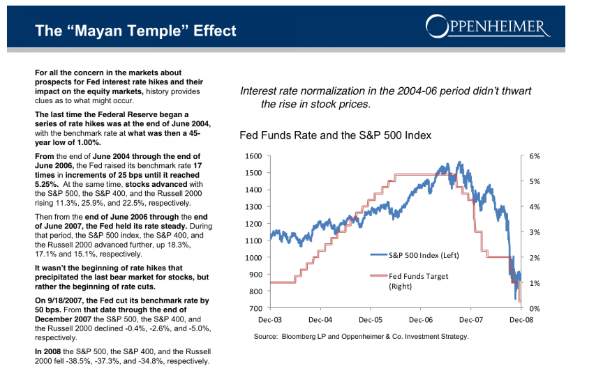
The Stock Market Bull Who Got 2014 Right Just Published This Fantastic Presentation I especially like the “Mayan Temple” effect, viz

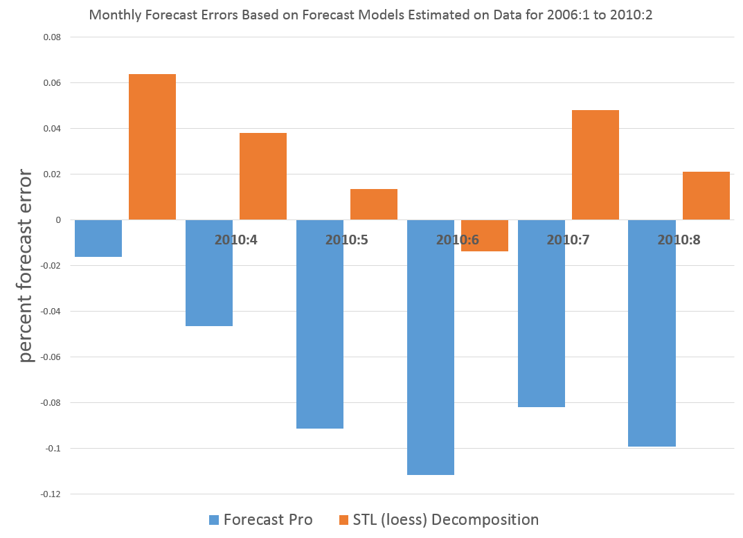
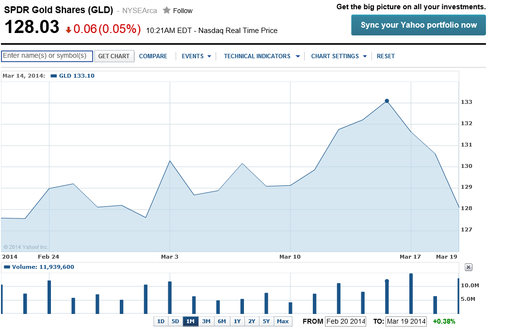
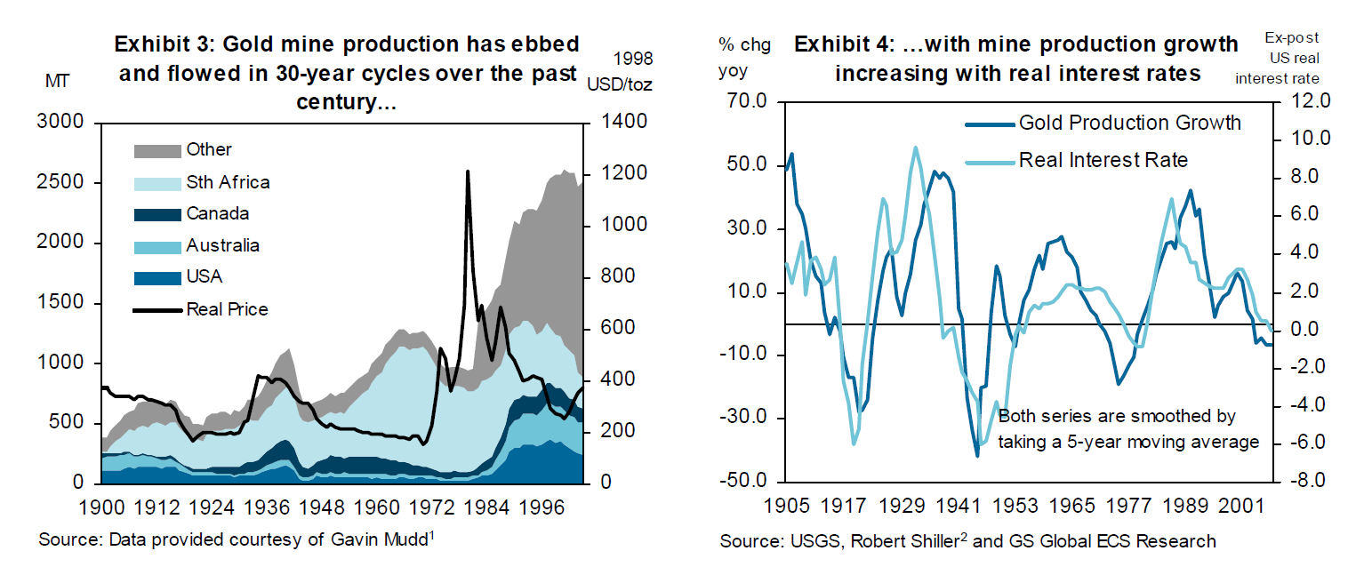
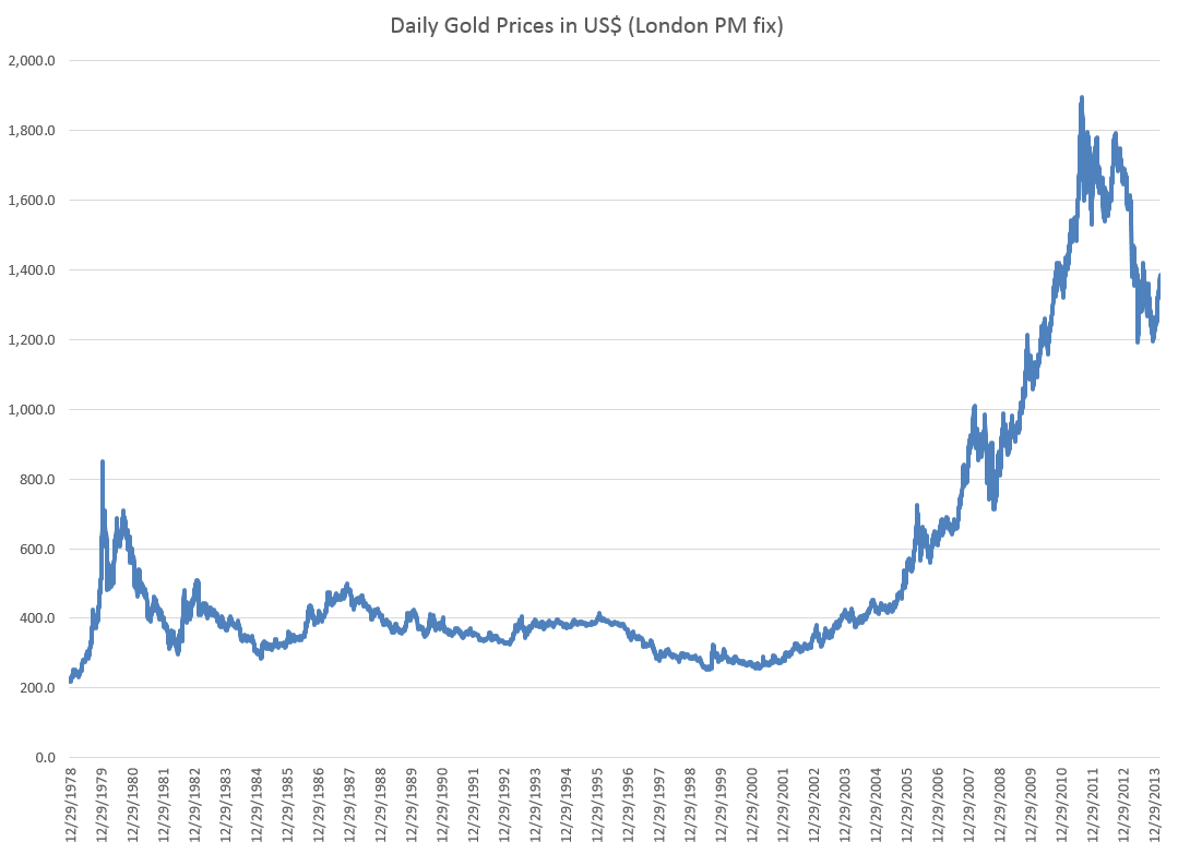
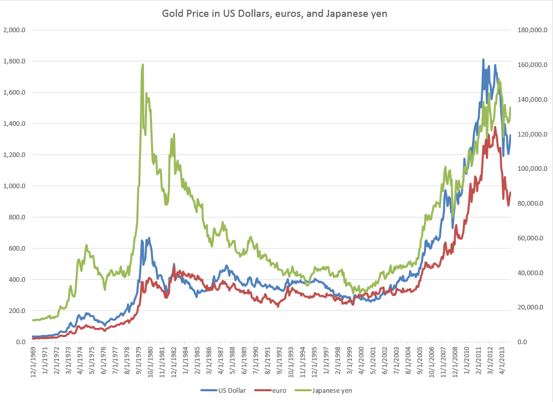
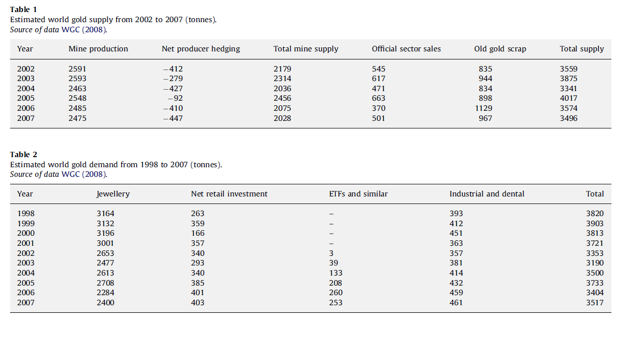
Why Gold & Oil Are Trading So Differently supply and demand – worth watching to keep primed on the key issues.

Technology

10 Astonishing Technologies On The Horizon – Some of these are pretty far-out, like teleportation which is now just gleam in the eye of quantum physicists, but some in the list are in prototype – like flying cars. Read more at Digital Journal entry on Business Insider.

Flexible and bendable smartphones
Smart jewelry
“Invisible” computers
Virtual shopping
Teleportation
Interplanetary Internet
Flying cars
Grow human organs
Prosthetic eyes
Electronic tattoos

Albert Einstein’s Entire Collection of Papers, Letters is Now Online

Princeton University Press makes this available.

Practice Your French Comprehension

Olivier Grisel, Software Engineer, Inria – broad overview of machine learning technologies. Helps me that the slides are in English.

accuracy of forecasts, analytical software, gold price forecasting, locally weighted regression smoothing, machine learning

Loess Seasonal Decomposition as a Forecasting Tool

April 16, 2014 Clive Jones

I’ve applied something called loess decomposition to the London PM Fix gold series previously discussed in this blog.

This suggests insights missing from an application of Forecast Pro – a sort of standard in the automatic forecasting field.

Loess decomposition separates a time series into components – trend, seasonals, and residuals or remainder – based on locally weighted regression smoothing of the data.

I always wondered whether, in fact, there was a seasonal component to the monthly London PM fix time series.

Not every monthly or quarterly time series has credible seasonal components, of course.

The proof would seem to be in the pudding. If a program derives seasonal components for a time series, do those seasonal components improve forecasts? That seems to be the critical issue.

STL Decomposition

STL decomposition – seasonal trend decomposition based on loess – was proposed by Cleveland et al in an interesting-sounding publication called “The Journal of Official Statistics.” I found the citation working through the procedure for bagging exponential smoothing mentioned in the previous post.

Amazingly, there is an online resource which calculates this loess decomposition for data you input, based on a listed R routine. The citation is Wessa P., (2013), Decomposition by Loess (v1.0.2) in Free Statistics Software (v1.1.23-r7), Office for Research Development and Education, URL http://www.wessa.net/rwasp_decomposeloess.wasp/

Comparison of STL Decomposition and Forecast Pro Gold Price Forecasts

Here’s a typical graph comparing the forecast errors from the Forecast Pro runs with STL Decomposition.

The trend component extracted by the STL decomposition was uncomplicated and easy to forecast by linear extrapolation. I added the seasonal component to these extrapolations to get the monthly forecasts over the six month forecast horizon. Forecast Pro, on the other hand, did not signal the existence of a seasonal component in this series, and, furthermore, identified the optimal forecast model as a random walk and the optimal forecast as the last observed value.

Here is the trend component from the STL decomposition.

Discussion

Potentially, there is lots more to discuss here.

For example, to establish forecasts based on the loess decomposition of the gold price outperform Forecast Pro means compiling a large number of forecast comparisons, ideally one for all possible training sets beyond a minimum number of observations required for stable calculation of the STL algorithm. That is, each training set generates somewhat different values for the trend, seasonals, and residuals with loess decomposition. And Forecast Pro needs to be run for all these possible training sets also, with forecasts compared to out-of-sample data.

While I have not gone to this extent, I have done these computations several times with good results for STL decomposition.

Also, it’s clear that loess decomposition extracts constant variance seasonals. However, the shape of these seasonals change as the training set changes. It is necessary, thus, to study whether these changes can reflect multiplicative seasonality, for series in which that type of seasonality predominates. For example, perhaps STL seasonals tend to reflect the end points of the training sets.

Bergmeir, Hyndman, and Benıtez (BHB) apply a Box Cox transformation in one of their bagged exponential smoothing methods. This is possibly another way to sidestep problems of multiplicative or hetereoskedastic seasonality. It also makes sense when one is attempting to bag a time series.

However, my explorations suggest the results of STL decomposition are quite flexible, and, in the case of this gold price series, often produce superior forecasts to results from one of the main off-the-shelf automatic forecasting programs.

I personally am going to work on including STL decomposition in my forecasting toolkit.

gold price forecasting, inflation, Janet Yellen outlook, long term forecasting, multivariate modeling

Forecasting the Price of Gold – 3

March 20, 2014 Clive Jones

Ukraine developments and other counter-currents, such as Janet Yellen’s recent comments, highlight my final topic on gold price forecasting – multivariate gold price forecasting models.

On the one hand, there has been increasing uncertainty as a result of Ukrainian turmoil, counterbalanced today by the reaction to the seemingly hawkish comments by Chairperson Janet Yellen of the US Federal Reserve Bank.

Traditionally, gold is considered a hedge against uncertainty. Indulge your imagination and it’s not hard to conjure up scary scenarios in the Ukraine. On the other hand, some interpret Yellen as signaling an earlier move to moving the Federal funds rate off zero, increasing interest rates, and, in the eyes of the market, making gold more expensive to hold.

Multivariate Forecasting Models of Gold Price – Some Considerations

It’s this zoo of factors and influences that you have to enter, if you want to try to forecast the price of gold in the short or longer term.

Variables to consider include inflation, exchange rates, gold lease rates, interest rates, stock market levels and volatility, and political uncertainty.

A lot of effort has been devoted to proving or attempting to question that gold is a hedge against inflation.

The bottom line appears to be that gold prices rise with inflation – over a matter of decades, but in shorter time periods, intervening factors can drive the real price of gold substantially away from a constant relationship to the overall price level.

Real (and possibly nominal) interest rates are a significant influence on gold prices in shorter time periods, but this relationship is complex. My reading of the literature suggests a better understanding of the supply side of the picture is probably necessary to bring all this into focus.

The Goldman Sachs Global Economics Paper 183 – Forecasting Gold as a Commodity – focuses on the supply side with charts such as the following –

The story here is that gold mine production responds to real interest rates, and thus the semi-periodic fluctuations in real interest rates are linked with a cycle of growth in gold production.

The Goldman Sachs Paper 183 suggests that higher real interest rates speed extraction, since the opportunity cost of leaving ore deposits in the ground increases. This is indeed the flip side of the negative impact of real interest rates on investment.

And, as noted in an earlier post,the Goldman Sachs forecast in 2010 proved prescient. Real interest rates have remained low since that time, and gold prices drifted down from higher levels at the end of the last decade.

Elasticities

Elasticities of response in a regression relationship show how percentage changes in the dependent variable – gold prices in this case – respond to percentage changes in, for example, the price level.

For gold to be an effective hedge against inflation, the elasticity of gold price with respect to changes in the price level should be approximately equal to 1.

This appears to be a credible elasticity for the United States, based on two studies conducted with different time spans of gold price data.

These studies are Gold as an Inflation Hedge? and the more recent Does Gold Act As An Inflation Hedge in the US and Japan. Also, a Gold Council report, Short-run and long-run determinants of the price of gold, develops a competent analysis.

These studies explore the cointegration of gold prices and inflation. Cointegration of unit root time series is an alternative to first differencing to reduce such time series to stationarity.

Thus, it’s not hard to show strong evidence that standard gold price series are one type or another of a random walk. Accordingly, straight-forward regression analysis of such series can easily lead to spurious correlation.

You might, for example, regress the price of gold onto some metric of the cumulative activity of an amoeba (characterized by Brownian motion) and come up with t-statistics that are, apparently, statistically significant. But that would, of course, be nonsense, and the relationship could evaporate with subsequent movements of either series.

So, the better research always gives consideration to the question of whether the variables in the models are, first of all, nonstationary OR whether there are cointegrated relationships.

While I am on the topic literature, I have to recommend looking at Theories of Gold Price Movements: Common Wisdom or Myths? This appears in the Wesleyan University Undergraduate Economic Review and makes for lively reading.

Thus, instead of viewing gold as a special asset, the authors suggest it is more reasonable to view gold as another currency, whose value is a reflection of the value of U.S. dollar.

The authors consider and reject a variety of hypotheses – such as the safe haven or consumer fear motivation to hold gold. They find a very significant relationship between the price movement of gold, real interest rates and the exchange rate, suggesting a close relationship between gold and the value of U.S. dollar. The multiple linear regressions verify these findings.

The Bottom Line

Over relatively long time periods – one to several decades – the price of gold moves more or less in concert with measures of the price level. In the shorter term, forecasting faces serious challenges, although there is a literature on the multivariate prediction of gold prices.

One prediction, however, seems reasonable on the basis of this review. Real interest rates should rise as the US Federal Reserve backs off from quantitative easing and other central banks around the world follow suit. Thus, increases in real interest rates seem likely at some point in the next few years. This seems to indicate that gold mining will strive to increase output, and perhaps that gold mining stocks might be a play.

accuracy of forecasts, ARIMA models, precious metals prices, predictive analytics, time series forecasting

Forecasting the Price of Gold – 2

March 18, 2014 Clive Jones

Searching “forecasting gold prices” on Google lands on a number of ARIMA (autoregressive integrated moving average) models of gold prices. Ideally, researchers focus on shorter term forecast horizons with this type of time series model.

I take a look at this approach here, moving onto multivariate approaches in subsequent posts.

Stylized Facts

These ARIMA models support stylized facts about gold prices such as: (1) gold prices constitute a nonstationary time series, (2) first differencing can reduce gold price time series to a stationary process, and, usually, (3) gold prices are random walks.

For example, consider daily gold prices from 1978 to the present.

This chart, based World Gold Council data and the London PM fix, shows gold prices do not fluctuate about a fixed level, but can move in patterns with a marked trend over several years.

The trick is to reduce such series to a mean stationary series through appropriate differencing and, perhaps, other data transformations, such as detrending and taking out seasonal variation. Guidance in this is provided by tools such as the autocorrelation function (ACF) and partial autocorrelation function (PACF) of the time series, as well as tests for unit roots.

Some Terminology

I want to talk about specific ARIMA models, such as ARIMA(0,1,1) or ARIMA(p,d,q), so it might be a good idea to review what this means.

Quickly, ARIMA models are described by three parameters: (1) the autoregressive parameter p, (2) the number of times d the time series needs to be differenced to reduce it to a mean stationary series, and (3) the moving average parameter q.

ARIMA(0,1,1) indicates a model where the original time series y_t is differenced once (d=1), and which has one lagged moving average term.

If the original time series is y_t, t=1,2,..n, the first differenced series is z_t=y_t-y_t-1, and an ARIMA(0,1,1) model looks like,

z_t = θ₁ε_t-1

or converting back into the original series yt,

y_t = μ + y_t-1 + θ₁ε_t-1

This is a random walk process with a drift term μ, incidentally.

As a note in the general case, the p and q parameters describe the span of the lags and moving average terms in the model. This is often done with backshift operators L_k(click to enlarge)

So you could have a sum of these backshift operators of different orders operating against y_t or z_t to generate a series of lags of order p. Similarly a sum of backshift operators of order q can operate against the error terms at various times. This supposedly provides a compact way of representing the general model with p lags and q moving average terms.

Similar terminology can indicate the nature of seasonality, when that is operative in a time series.

These parameters are determined by considering the autocorrelation function ACF and partial autocorrelation function PACF, as well as tests for unit roots.

I’ve seen this referred to as “reading the tea leaves.”

Gold Price ARIMA models

I’ve looked over several papers on ARIMA models for gold prices, and conducted my own analysis.

My research confirms that the ACF and PACF indicates gold prices (of course, always defined as from some data source and for some trading frequency) are, in fact, random walks.

So this means that we can take, for example, the recent research of Dr. M. Massarrat Ali Khan of College of Computer Science and Information System, Institute of Business Management, Korangi Creek, Karachi as representative in developing an ARIMA model to forecast gold prices.

Dr. Massarrat’s analysis uses daily London PM fix data from January 02, 2003 to March 1, 2012, concluding that an ARIMA(0,1,1) has the best forecasting performance. This research also applies unit root tests to verify that the daily gold price series is stationary, after first differencing. Significantly, an ARIMA(1,1,0) model produced roughly similar, but somewhat inferior forecasts.

I think some of the other attempts at ARIMA analysis of gold price time series illustrate various modeling problems.

For example there is the classic over-reach of research by Australian researchers in An overview of global gold market and gold price forecasting. These academics identify the nonstationarity of gold prices, but attempt a ten year forecast, based on a modeling approach that incorporates jumps as well as standard ARIMA structure.

A new model proposed a trend stationary process to solve the nonstationary problems in previous models. The advantage of this model is that it includes the jump and dip components into the model as parameters. The behaviour of historical commodities prices includes three differ- ent components: long-term reversion, diffusion and jump/dip diffusion. The proposed model was validated with historical gold prices. The model was then applied to forecast the gold price for the next 10 years. The results indicated that, assuming the current price jump initiated in 2007 behaves in the same manner as that experienced in 1978, the gold price would stay abnormally high up to the end of 2014. After that, the price would revert to the long-term trend until 2018.

As the introductory graph shows, this forecast issued in 2009 or 2010 was massively wrong, since gold prices slumped significantly after about 2012.

So much for long-term forecasts based on univariate time series.

Summing Up

I have not referenced many ARIMA forecasting papers relating to gold price I have seen, but focused on a couple – one which “gets it right” and another which makes a heroically wrong but interesting ten year forecast.

Gold prices appear to be random walks in many frequencies – daily, monthly average, and so forth.

Attempts at superimposing long term trends or even jump patterns seem destined to failure.

However, multivariate modeling approaches, when carefully implemented, may offer some hope of disentangling longer term trends and changes in volatility. I’m working on that post now.

ARIMA models, currency forecasts, financial forecasting, global business forecasts, gold price forecasting, predictive analytics, random walk

Forecasting the Price of Gold – 1

March 17, 2014 Clive Jones

I’m planning posts on forecasting the price of gold this week. This is an introductory post.

The Question of Price

What is the “price” of gold, or, rather, is there a single, integrated global gold market?

This is partly an anthropological question. Clearly in some locales, perhaps in rural India, people bring their gold jewelry to some local merchant or craftsman, and get widely varying prices. Presumably, though this merchant negotiates with a broker in a larger city of India, and trades at prices which converge to some global average. Very similar considerations apply to interest rates, which are significantly higher at pawnbrokers and so forth.

The World Gold Council uses the London PM fix, which at the time of this writing was $1,379 per troy ounce.

The Wikipedia article on gold fixing recounts the history of this twice daily price setting, dating back, with breaks for wars, to 1919.

One thing is clear, however. The “price of gold” varies with the currency unit in which it is stated. The World Gold Council, for example, supplies extensive historical data upon registering with them. Here is a chart of the monthly gold prices based on the PM or afternoon fix, dating back to 1970.

Another insight from this chart is that the price of gold may be correlated with the price of oil, which also ramped up at the end of the 1970’s and again in 2007, recovering quickly from the Great Recession in 2008-09 to surge up again by 2010-11.

But that gets ahead of our story.

The Supply and Demand for Gold

Here are two valuable tables on gold supply and demand fundamentals, based on World Gold Council sources, via an An overview of global gold market and gold price forecasting. I’ve more to say about the forecasting model in that article, but the descriptive material is helpful (click to enlarge).

These tables give an idea of the main components of gold supply and demand over a several years recently.

Gold is an unusual commodity in that one of its primary demand components – jewelry – can contribute to the supply-side. Thus, gold is in some sense renewable and recyclable.

Table 1 above shows the annual supplies in this period in the last decade ran on the order of three to four thousand tonnes, where a tonne is 2,240 pounds and equal conveniently to 1000 kilograms.

Demand for jewelry is a good proportion of this annual supply, with demands by ETF’s or exchange traded funds rising rapidly in this period. The industrial and dental demand is an order of magnitude lower and steady.

One of the basic distinctions is between the monetary versus nonmonetary uses or demands for gold.

In total, central banks held about 30,000 tonnes of gold as reserves in 2008.

Another estimated 30,000 tonnes was held in inventory for industrial uses, with a whopping 100,000 tonnes being held as jewelry.

India and China constitute the largest single countries in terms of consumer holdings of gold, where it clearly functions as a store of value and hedge against uncertainty.

Gold Market Activity

In addition to actual purchases of gold, there are gold futures. The CME Group hosts a website with gold future listings. The site states,

Gold futures are hedging tools for commercial producers and users of gold. They also provide global gold price discovery and opportunities for portfolio diversification. In addition, they: Offer ongoing trading opportunities, since gold prices respond quickly to political and economic events, Serve as an alternative to investing in gold bullion, coins, and mining stocks

Some of these contracts are recorded at exchanges, but it seems the bulk of them are over-the-counter.

A study by the London Bullion Market Association estimates that 10.9bn ounces of gold, worth $15,200bn, changed hands in the first quarter of 2011 just in London’s markets. That’s 125 times the annual output of the world’s gold mines – and twice the quantity of gold that has ever been mined.

The Forecasting Problem

The forecasting problem for gold prices, accordingly, is complex. Extant series for gold prices do exist and underpin a lot of the market activity at central exchanges, but the total volume of contracts and gold exchanging hands is many times the actual physical quantity of the product. And there is a definite political dimension to gold pricing, because of the monetary uses of gold and the actions of central banks increasing and decreasing their reserves.

But the standard approaches to the forecasting problem are the same as can be witnessed in any number of other markets. These include the usual time series methods, focused around arima or autoregressive moving average models and multivariate regression models. More up-to-date tactics revolve around tests of cointegration of time series and VAR models. And, of course, one of the fundamental questions is whether gold prices in their many incarnations are best considered to be a random walk.

Business Forecasting