Tag Archives: predictive analytics

Big Data, data science, financial forecasting, many predictors, predictive analytics, the LASSO, variable selection

Variable Selection Procedures – The LASSO

March 4, 2014 Clive Jones

The LASSO (Least Absolute Shrinkage and Selection Operator) is a method of automatic variable selection which can be used to select predictors X* of a target variable Y from a larger set of potential or candidate predictors X.

Developed in 1996 by Tibshirani, the LASSO formulates curve fitting as a quadratic programming problem, where the objective function penalizes the absolute size of the regression coefficients, based on the value of a tuning parameter λ. In doing so, the LASSO can drive the coefficients of irrelevant variables to zero, thus performing automatic variable selection.

This post features a toy example illustrating tactics in variable selection with the lasso. The post also dicusses the issue of consistency – how we know from a large sample perspective that we are honing in on the true set of predictors when we apply the LASSO.

My take is a two-step approach is often best. The first step is to use the LASSO to identify a subset of potential predictors which are likely to include the best predictors. Then, implement stepwise regression or other standard variable selection procedures to select the final specification, since there is a presumption that the LASSO “over-selects” (Suggested at the end of On Model Selection Consistency of Lasso).

Toy Example

The LASSO penalizes the absolute size of the regression coefficients, based on the value of a tuning parameter λ. When there are many possible predictors, many of which actually exert zero to little influence on a target variable, the lasso can be especially useful in variable selection.

For example, generate a batch of random variables in a 100 by 15 array – representing 100 observations on 15 potential explanatory variables. Mean-center each column. Then, determine coefficient values for these 15 explanatory variables, allowing several to have zero contribution to the dependent variable. Calculate the value of the dependent variable y for each of these 100 cases, adding in a normally distributed error term.

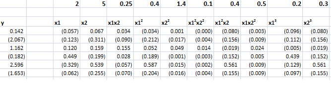
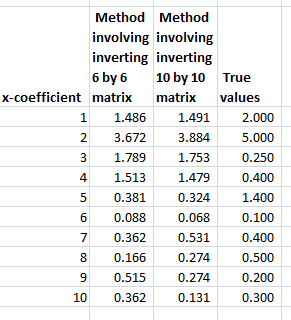
The following Table illustrates something of the power of the lasso.

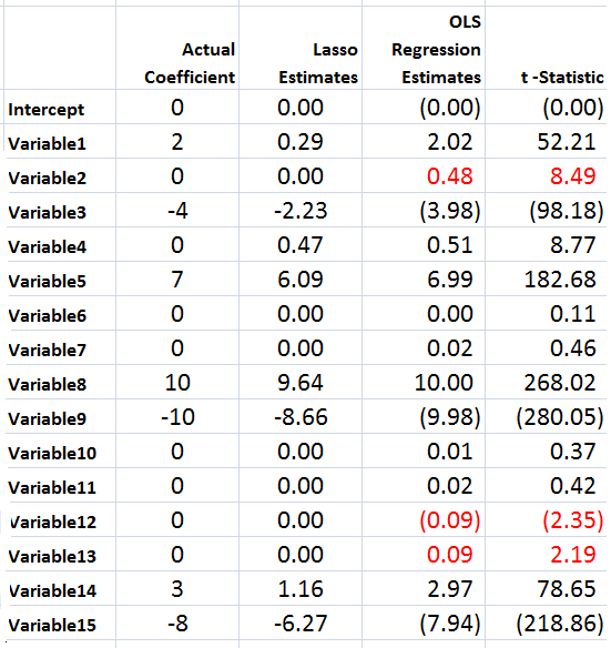
Using the Matlab lasso procedure and a lambda value of 0.3, seven of the eight zero coefficients are correctly identified. The OLS regression estimate, on the other hand, indicates that three of the zero coefficients are nonzero at a level of 95 percent statistical significance or more (magnitude of the t-statistic > 2).

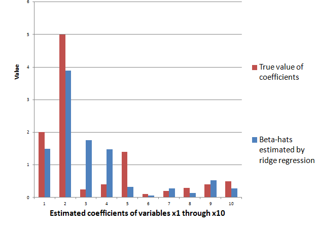
Of course, the lasso also shrinks the value of the nonzero coefficients. Like ridge regression, then, the lasso introduces bias to parameter estimates, and, indeed, for large enough values of lambda drives all coefficient to zero.

Note OLS can become impossible, when the number of predictors in X* is greater than the number of observations in Y and X. The LASSO, however, has no problem dealing with many predictors.

Real World Examples

For a recent application of the lasso, see the Dallas Federal Reserve occasional paper Hedge Fund Dynamic Market Stability. Note that the lasso is used to identify the key drivers, and other estimation techniques are employed to hone in on the parameter estimates.

For an application of the LASSO to logistic regression in genetics and molecular biology, see Lasso Logistic Regression, GSoft and the Cyclic Coordinate Descent Algorithm, Application to Gene Expression Data. As the title suggests, this illustrates the use of the lasso in logistic regression, frequently utilized in biomedical applications.

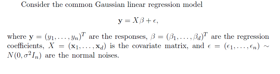
Formal Statement of the Problem Solved by the LASSO

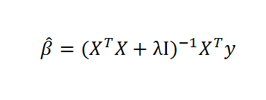
The objective function in the lasso involves minimizing the residual sum of squares, the same entity figuring in ordinary least squares (OLS) regression, subject to a bound on the sum of the absolute value of the coefficients. The following clarifies this in notation, spelling out the objective function.

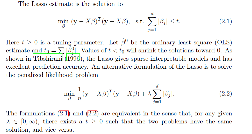
The computation of the lasso solutions is a quadratic programming problem, tackled by standard numerical analysis algorithms. For an analytical discussion of the lasso and other regression shrinkage methods, see the outstanding free textbook The Elements of Statistical Learning by Hastie, Tibshirani, and Friedman.

The Issue of Consistency

The consistency of an estimator or procedure concerns its large sample characteristics. We know the LASSO produces biased parameter estimates, so the relevant consistency is whether the LASSO correctly predicts which variables from a larger set are in fact the predictors.

In other words, when can the LASSO select the “true model?”

Now in the past, this literature is extraordinarily opaque, involving something called the Irrepresentable Condition, which can be glossed as –

almost necessary and sufficient for Lasso to select the true model both in the classical fixed p setting and in the large p setting as the sample size n gets large…This Irrepresentable Condition, which depends mainly on the covariance of the predictor variables, states that Lasso selects the true model consistently if and (almost) only if the predictors that are not in the true model are “irrepresentable” (in a sense to be clarified) by predictors that are in the true model.

Fortunately a ray of light has burst through with Assumptionless Consistency of the Lasso by Chatterjee. Apparently, the LASSO selects the true model almost always – with minimal side assumptions – providing we are satisfied with the prediction error criterion – the mean square prediction error – employed in Tibshirani’s original paper.

Finally, cross-validation is typically used to select the tuning parameter λ, and is another example of this procedure highlighted by Varian’s recent paper.

Big Data, data mining, data science, kernel ridge regression

Kernel Ridge Regression – A Toy Example

March 1, 2014 Clive Jones

Kernel ridge regression (KRR) is a promising technique in forecasting and other applications, when there are “fat” databases. It’s intrinsically “Big Data” and can accommodate nonlinearity, in addition to many predictors.

Kernel ridge regression, however, is shrouded in mathematical complexity. While this is certainly not window-dressing, it can obscure the fact that the method is no different from ordinary ridge regression on transformations of regressors, except for an algebraic trick to improve computational efficiency.

This post develops a spreadsheet example illustrating this key point – kernel ridge regression is no different from ordinary ridge regression…except for an algebraic trick.

Background

Most applications of KRR have been in the area of machine learning, especially optical character recognition.

To date, the primary forecasting application involves a well-known “fat” macroeconomic database. Using this data, researchers from the Tinbergen Institute and Erasmus University develop KRR models which outperform principal component regressions in out-of-sample forecasts of variables, such as real industrial production and employment.

You might want to tab and review several white papers on applying KRR to business/economic forecasting, including,

Nonlinear Forecasting with Many Predictors using Kernel Ridge Regression

Modelling Issues in Kernel Ridge Regression

Model Selection in Kernel Ridge Regression

This research holds out great promise for KRR, concluding, in one of these selections that,

The empirical application to forecasting four key U.S. macroeconomic variables — production, income, sales, and employment — shows that kernel-based methods are often preferable to, and always competitive with, well-established autoregressive and principal-components-based methods. Kernel techniques also outperform previously proposed extensions of the standard PC-based approach to accommodate nonlinearity.

Calculating a Ridge Regression (and Kernel Ridge Regression)

Recall the formula for ridge regression,

Here, X is the data matrix, X^Tis the transpose of X, λ is the conditioning factor, I is the identify matrix, and y is a vector of values of the dependent or target variable. The “beta-hats” are estimated β’s or coefficient values in the conventional linear regression equation,

y = β₁x₁+ β₂x₂+… β_Nx_N

The conditioning factor λ is determined by cross-validation or holdout samples (see Hal Varian’s discussion of this in his recent paper).

Just for the record, ridge regression is a data regularization method which works wonders when there are glitches – such as multicollinearity – which explode the variance of estimated coefficients.

Ridge regression, and kernel ridge regression, also can handle the situation where there are more predictors or explanatory variables than cases or observations.

A Specialized Dataset

Now let us consider ridge regression with the following specialized dataset.

By construction, the equation,

y = 2x₁ + 5x₂+0.25x₁x₂+0.5x₁²+1.5x₂²+0.5x₁x₂²+0.4x₁²x₂+0.2x₁³+0.3x₂³

generates the six values of y from the sums of ten terms in x1 and x2, their powers, and cross-products.

Although we really only have two explanatory variables, x₁ and x_2,the equation, as a sum of 10 terms, can be considered to be constructed out of ten, rather than two, variables.

However, adopting this convenience, it means we have more explanatory variables (10) than observations on the dependent variable (6).

Thus, it will be impossible to estimate the beta’s by OLS.

Of course, we can develop estimates of the values of the coefficients of the true relationship between y and the data on the explanatory variables with ridge regression.

Then, we will find that we can map all ten of these apparent variables in the equation onto a kernel of two variables, simplifying the matrix computations in a fundamental way, using this so-called algebraic trick.

The ordinary ridge regression data matrix X is 6 rows by 10 columns, since there are six observations or cases and ten explanatory variables. Thus, the transpose X^T is a 10 by 6 matrix. Accordingly, the product X^TX is a 10 by 10 matrix, resulting in a 10 by 10 inverse matrix after the conditioning factor and identity matrix is added in to X^TX.

In fact, the matrix equation for ridge regression can be calculated within a spreadsheet using the Excel functions mmult(.,) and minverse() and the transpose operation from Copy. The conditioning factor λ can be determined by trial and error, or by writing a Visual Basic algorithm to explore the mean square error of parameter values associated with different values λ.

The ridge regression formula above, therefore, gives us estimates for ten beta-hats, as indicated in the following chart, using a λ or conditioning coefficient of .005.

The red bars indicate the true coefficient values, and the blue bars are the beta-hats estimated by the ridge regression formula.

As you can see, ridge regression “gets in the ballpark” in terms of the true values of the coefficients of this linear expression. However, with only 6 observations, the estimate is highly approximate.

The Kernel Trick

Now with suitable pre- and post-multiplications and resorting, it is possible to switch things around to another matrix formula,

Exterkate et al show the matrix algebra in a section of their “Nonlinear..” white paper using somewhat different symbolism.

Key point – the matrix formula listed just above involves inverting a smaller matrix, than the original formula – in our example, a 6 by 6, rather than a 10 by 10 matrix.

The following Table shows the beta-hats estimated by these two formulas are similar and compares them with the “true” values of the coefficients.

Differences in the estimates by these formally identical formulas relate strictly to issues at the level of numerical analysis and computation.

Kernels

Notice that the ten variables could correspond to a Taylor expansion which might be used to estimate the value of a nonlinear function. This is a key fact and illustrates the concept of a “kernel”.

Thus, designating K = XX^T_,we find that the elements of K can be obtained without going through the indicated multiplication of these two matrices. This is because K is a polynomial kernel.

There is a great deal more that can be said about this example and the technique in general. Two big areas are (a) arriving at the estimate of the conditioning factor λ and (b) discussing the range of possible kernels that can be used, what makes a kernel a kernel, how to generate kernels from existing kernels, where Hilbert spaces come into the picture, and so forth.

But hopefully this simple example can point the way.

For additional insight and the source for the headline Homer Simpson graphic, see The Kernel Trick.

analytical software, Big Data, Chinese economy, data mining, data science, developing country forecast

Links – February 28

February 28, 2014 Clive Jones

Data Science and Predictive Analytics

Data Scientists Predict Oscar® Winners Again; Social Media May Love Leo, But Data Says “No”

..the data shows that Matthew McConaughey will win best actor for his role in the movie Dallas Buyers Guide; Alfonso Cuaron will win best director for the movie Gravity; and 12 Months a Slave will win the coveted prize for best picture – which is the closest among all the races. The awards will not be a clean sweep for any particular picture, although the other award winners are expected to be Jared Leto for best supporting actor in Dallas Buyers Club; Cate Blanchet for best actress in Blue Jasmine; and Lupita Nyong’o for best supporting actress in 12 Years a Slave.

10 Most Influential Analytics Leaders in India

Pankaj Kulshreshtha – Business Leader, Analytics & Research at Genpact

Rohit Tandon – Vice President, Strategy WW Head of HP Global Analytics

Sameer Dhanrajani – Business Leader, Cognizant Analytics

Srikanth Velamakanni – Co founder and Chief Executive Officer at Fractal Analytics

Pankaj Rai – Director, Global Analytics at Dell

Amit Khanna – Partner at KPMG

Ashish Singru – Director eBay India Analytics Center

Arnab Chakraborty – Managing Director, Analytics at Accenture Consulting

Anil Kaul – CEO and Co-founder at Absolutdata

Dr. N.R.Srinivasa Raghavan, Senior Vice President & Head of Analytics at Reliance Industries Limited

Interview with Jörg Kienitz, co-author with Daniel Wetterau of Financial Modelling: Theory, Implementation and Practice with MATLAB Source

JB: Why MATLAB? Was there a reason for choosing it in this context?

JK: Our attitude was that it was a nice environment for developing models because you do not have to concentrate on the side issues. For instance, if you want to calibrate a model you can really concentrate on implementing the model without having to think about the algorithms doing the optimisation for example. MATLAB offers a lot of optimisation routines which are really reliable and which are fast, which are tested and used by thousands of people in the industry. We thought it was a good idea to use standardised mathematical software, a programming language where all the mathematical functions like optimisation, like Fourier transform, random number generator and so on, are very reliable and robust. That way we could concentrate on the algorithms which are necessary to implement models, and not have to worry about a programming a random number generator or such stuff. That was the main idea, to work on a strong ground and build our house on a really nice foundation. So that was the idea of choosing MATLAB.

Knowledge-based programming: Wolfram releases first demo of new language, 30 years in the making

Economy

Credit Card Debt Threatens Turkey’s Economy – kind of like the subprime mortgage scene in the US before 2008.

..Standard & Poor’s warned in a report last week that the boom in consumer credit had become a serious risk for Turkish lenders. Slowing economic growth, political turmoil and increasing reluctance by foreign investors to provide financing “are prompting a deterioration in the operating environment for Turkish banks,”

A shadow banking map from the New York Fed. Go here and zoom in for detail.

China Sees Expansion Outweighing Yuan, Shadow Bank Risk

China’s Finance Minister Lou Jiwei played down yuan declines and the risks from shadow banking as central bank Governor Zhou Xiaochuan signaled that the nation’s economy can sustain growth of between 7 percent and 8 percent.

Outer Space

715 New Planets Found (You Read That Number Right)

Speaks for itself. That’s a lot of new planets. One of the older discoveries – Tau Boötis b – has been shown to have water vapor in its atmosphere.

Hillary, ‘The Family,’ and Uganda’s Anti-Gay Christian Mafia

I heard about this at the SunDance film gathering in 2013. Apparently, there are links between US and Ugandan groups in promulgating this horrific law.

An Astronaut’s View of the North Korean Electricity Black Hole

causal discovery, forecast competitions, Granger causality, predictive analytics

Causal Discovery

February 17, 2014 Clive Jones

So there’s a new kid on the block, really a former resident who moved back to the neighborhood with spiffy new toys – causal discovery.

Competitions and challenges give a flavor of this rapidly developing field – for example, the Causality Challenge #3: Cause-effect pairs, sponsored by a list of pre-eminent IT organizations and scientific societies (including Kaggle).

By way of illustration, B → A but A does not cause B – Why?

These data, as the flipped answer indicates, are temperature and altitude of German cities. So altitude causes temperature, but temperature obviously does not cause altitude.

The non-linearity in the scatter diagram is a clue. Thus, values of variable A above about 130 map onto more than one value of B, which is problematic from conventional definition of causality. One cause should not have two completely different effects, unless there are confounding variables.

It’s a little fuzzy, but the associated challenge is very interesting, and data pairs still are available.

We provide hundreds of pairs of real variables with known causal relationships from domains as diverse as chemistry, climatology, ecology, economy, engineering, epidemiology, genomics, medicine, physics. and sociology. Those are intermixed with controls (pairs of independent variables and pairs of variables that are dependent but not causally related) and semi-artificial cause-effect pairs (real variables mixed in various ways to produce a given outcome). This challenge is limited to pairs of variables deprived of their context.

Asymmetries As Clues to Causal Direction of Influence

The causal direction in the graph above is suggested by the non-invertibility of the functional relationship between B and A.

Another clue from reversing the direction of causal influence relates to the error distributions of the functional relationship between pairs of variables. This occurs when these error distributions are non-Gaussian, as Patrik Hoyer and others illustrate in Nonlinear causal discovery with additive noise models.

The authors present simulation and empirical examples.

Their first real-world example comes from data on eruptions of the Old Faithful geyser in Yellowstone National Park in the US.

Hoyer et al write,

The first dataset, the “Old Faithful” dataset [17] contains data about the duration of an eruption and the time interval between subsequent eruptions of the Old Faithful geyser in Yellowstone National Park, USA. Our method obtains a p-value of 0.5 for the (forward) model “current duration causes next interval length” and a p-value of 4.4 x 10^-9for the (backward) model “next interval length causes current duration”. Thus, we accept the model where the time interval between the current and the next eruption is a function of the duration of the current eruption, but reject the reverse model. This is in line with the chronological ordering of these events. Figure 3 illustrates the data, the forward and backward fit and the residuals for both fits. Note that for the forward model, the residuals seem to be independent of the duration, whereas for the backward model, the residuals are clearly dependent on the interval length.

Then, they too consider temperature and altitude pairings.

Here, the correct model – altitude causes temperature – results in a much more random scatter of residuals, than the reverse direction model.

Patrik Hoyer and Aapo Hyvärinen are a couple of names from this Helsinki group of researchers whose papers are interesting to read and review.

One of the early champions of this resurgence of interest in causality works from a department of philosophy – Peter Spirtes. It’s almost as if the discussion of causal theory were relegated to philosophy, to be revitalized by machine learning and Big Data:

The rapid spread of interest in the last three decades in principled methods of search or estimation of causal relations has been driven in part by technological developments, especially the changing nature of modern data collection and storage techniques, and the increases in the processing power and storage capacities of computers. Statistics books from 30 years ago often presented examples with fewer than 10 variables, in domains where some background knowledge was plausible. In contrast, in new domains such as climate research (where satellite data now provide daily quantities of data unthinkable a few decades ago), fMRI brain imaging, and microarray measurements of gene expression, the number of variables can range into the tens of thousands, and there is often limited background knowledge to reduce the space of alternative causal hypotheses. Even when experimental interventions are possible, performing the many thousands of experiments that would be required to discover causal relationships between thousands or tens of thousands of variables is often not practical. In such domains, non-automated causal discovery techniques from sample data, or sample data together with a limited number of experiments, appears to be hopeless, while the availability of computers with increased processing power and storage capacity allow for the practical implementation of computationally intensive automated search algorithms over large search spaces.

Introduction to Causal Inference

bagging, boosting, classification models, ensemble forecasts, random subspace ensemble methods

Random Subspace Ensemble Methods (Random Forest™ algorithm)

February 12, 2014 Clive Jones

As a term, random forests apparently is trademarked, which is, in a way, a shame because it is so evocative – random forests, for example, are comprised of a large number of different decision or regression trees, and so forth.

Whatever the name we use, however, the Random Forest™ algorithm is a powerful technique. Random subspace ensemble methods form the basis for several real world applications, such as Microsoft’s Kinect, facial recognition programs in cell phone and other digital cameras, and figure importantly in many Kaggle competitions, according to Jeremy Howard, formerly Kaggle Chief Scientist.

I assemble here a Howard talk from 2011 called “Getting In Shape For The Sport Of Data Science” and instructional videos from a data science course at the University of British Columbia (UBC). Watching these involves a time commitment, but it’s possible to let certain parts roll and then to skip ahead. Be sure and catch the last part of Howard’s talk, since he’s good at explaining random subspace ensemble methods, aka random forests.

It certainly helps me get up to speed to watch something, as opposed to reading papers on a fairly unfamiliar combination of set theory and statistics.

By way of introduction, the first step is to consider a decision tree. One of the UBC videos notes that decision trees faded from popularity some decades ago, but have come back with the emergence of ensemble methods.

So a decision tree is a graph which summarizes the classification of multi-dimensional points in some space, usually based on creating rectangular areas with reference to the coordinates. The videos make this clearer.

So this is nice, but decision trees of this sort tend to over-fit; they may not generalize very well. There are methods of “pruning” or simplification which can help generalization, but another tactic is to utilize ensemble methods. In other words, develop a bunch of decision trees classifying some set of multi-attribute items.

Random forests simply build such decision trees with a randomly selected group of attributes, subsets of the total attributes defining the items which need to be classified.

The idea is to build enough of these weak predictors and then average to arrive at a modal or “majority rule” classification.

Here’s the Howard talk.

Then, there is an introductory UBC video on decision trees

This video goes into detail on the method of constructing random forests.

Then the talk on random subspace ensemble applications.

Big Data, predicting crime, predictive analytics

Crime Prediction

January 19, 2014 Clive Jones

PredPol markets a crime prediction system tested in and currently used by Los Angeles, CA and Seattle, WA, and under evaluation elsewhere (London, UK). The product takes historic statistics and generates real-time predictions of where new crimes are likely to occur – within highly localized areas.

The spec sheet calls it “cloud-based, easy-to-use” software, offering this basic description.

This has generated lots of press and TV coverage.

In July 2013, there was a thoughtful article in the Economist Don’t even think about it and a piece on National Public Radio (NPR).

A YouTube video features a contribution from one of the company founders – Jeffrey Brantingham.

From what I glean, PredPol takes the idea of crime hotspots a step further, identifying behavioral patterns in burglaries and other property crimes – such as the higher probability of a repeat break-in, or increased probability of a break-in to a neighbor of a house that has been burglarized. Transportation access to and egress from crime sites is also important to criminals – the easier, the better.

The proof is in the pudding. And there have been reductions in property crime in locales where the PredPol system is being applied, although not necessarily increases in arrests. The rationale is that sending additional patrols into the targeted areas deters criminals.

Maybe some of these would-be criminals go elsewhere to rob and steal, but others may simply be deterred, given the criminal mind is at least partly motivated by sheer laziness.

Criticism of PredPol

I can think of several potential flaws.

Analytically, there have to be dynamic effects from the success of PredPol in any locale. If successful, in other words, the algorithm will change the crime pattern, and then what?
Also, there is a risk of sort of fooling oneself, if the lower crime stats are taken as evidence that the software is effective. Maybe crimes would have decreased anyway.
And there are constitutional issues, if police simply stop people to prevent their committing a crime before it has happened, based on the predictions of the software.

Last November, some of the first critical articles about PredPol came out, motivated in part by a SFWeekly article All Tomorrow’s Crimes: The Future of Policing Looks a Lot Like Good Branding

In the meantime, PredPol seems destined for wide application in larger urban areas, and is surely has some of the best PR of any implementation of Big Data and predictive analytics.

ARIMA models, Monte Carlo simulation, predictive analytics, stock market forecasts

Predicting the S&P 500 or the SPY Exchange-Traded Fund

January 12, 2014 Clive Jones 2 Comments

By some lights, predicting the stock market is the ultimate challenge. Tremendous resources are dedicated to it – pundits on TV, specialized trading programs, PhD’s doing high-end quantitative analysis in hedge funds. And then, of course, theories of “rational expectations” and “efficient markets” deny the possibility of any consistent success at stock market prediction, on grounds that stock prices are basically random walks.

I personally have not dabbled much in forecasting the market, until about two months ago, when I grabbed a bunch of data on the S&P 500 and tried some regressions with lags on S&P 500 daily returns and daily returns from the VIX volatility index.

What I discovered is completely replicable, and also, so far as I can see, is not widely known.

An autoregressive time series model of S&P 500 or SPY daily returns, built with data from 1993 to early 2008, can outperform a Buy & Hold strategy initiated with out-of-sample data beginning January 2008 and carrying through to recent days.

Here is a comparison of cumulative gains from a Buy & Hold strategy initiated January 23, 2008 with a Trading Strategy informed by my autoregressive (AR) model.

So, reading this chart, investing $1000 January 23, 2008 and not touching this investment leads to cumulative returns of $1586.84 – that’s the Buy & Hold strategy.

The AR trading model, however, generates cumulative returns over this period of $2097.

The trading program based on the autoregressive model I am presenting here works like this. The AR model predicts the next day return for the SPY, based on the model coefficients (which I detail below) and the daily returns through the current day. So, if there is an element of unrealism, it is because the model is based on the daily returns computed on closing values day-by-day. But, obviously, you have to trade before the closing bell (in standard trading), so you need to use a estimate of the current day’s closing value obtained very close to the bell, before deciding whether to invest, sell, or buy SPY for the next day’s action.

But basically, assuming we can do this, perhaps seconds before the bell, and come close to an estimate of the current day closing price – the AR trading program is to buy SPY if the next day’s return is predicted to be positive – or if you currently hold SPY, to continue holding it. If the next day’s return is predicted to be negative, you sell your holdings.

It’s as simple as that.

So the AR model predicts daily returns on a one-day-ahead basis, using information on daily returns through the current trading day, plus the model coefficients.

Speaking of which, here are the coefficients from the Matlab “printout.”

There are a couple of nuances here. First, these parameter values do not derive from an ordinary least squares (OLS) regression. Instead, they are produced by maximum likelihood estimation, assuming the underlying distribution is a t-distribution (not a Gaussian distribution).

The use of a t-distribution, the idea of which I got to some extent from Nassim Taleb’s new text-in-progress mentioned two posts ago, is motivated by the unusual distribution of residuals of an OLS regression of lagged daily returns.

The proof is in the pudding here, too, since the above coefficients work better than ones developed on the (manifestly incorrect) assumption that the underlying error distribution is Gaussian.

Here is a graph of the 30-day moving averages of the proportion of signs of daily returns correctly predicted by this model.

Overall, about 53 percent of the signs of the daily returns in this out-of-sample period are predicted correctly.

If you look at this graph, too, it’s clear there are some differences in performance over this period. Thus, the accuracy of the model took a dive in 2009, in the depths of the Great Recession. And, model performance achieved significantly higher success proportions in 2012 and early 2013, perhaps related to markets getting used to money being poured in by the Fed’s policies of quantitative easing.

Why This AR Model is Such a Big Deal

I find it surprising that a set of fixed coefficients applied to the past 30 values of the SPY daily returns continue to predict effectively, months and years after the end of the in-sample values.

And, I might add, it’s not clear that updating the AR model always improves the outcomes, although I can do more work on this and also on the optimal sample period generally.

Can this be a matter of pure chance? This has to be considered, but I don’t think so. Monte Carlo simulations of randomized trading indicate that there is a 95 percent chance or better than returns of $2097 in this period are not due to chance. In other words, if I decide to trade on a day based on a flip of a fair coin, heads I buy, tails I sell at the end of the day, it’s highly unlikely I will generate cumulative returns of $2097, given the SPY returns over this period.

The performance of this trading model holds up fairly well through December of last year, but degrades some in the first days of 2014.

I think this is a feather in the cap of forecasting, so to speak. Also, it seems to me that economists promoting ideas of market efficiency and rational expectations need to take these findings into account. Everything is extant. I have provided the coefficients. You can get the SPY daily return values from Yahoo Finance. You can calculate everything yourself to check. I’ve done this several times, slightly differently each time. This time I used Matlab, and its arima estimation procedures work well.

I’m not quite sure what to make of all this, but I think it’s important. Naturally, I am extending these results in my personal model-building, and I can report that extensions are possible. At the same time, no extension of this model I have seen achieves more than nearly 60 percent accuracy in predicting the direction of change or sign of the daily returns, so you are going to lose money sometimes applying these models. Day-trading is a risky business.

Business Forecasting