Because the Great Recession of 2008-2009 was closely tied with asset bubbles in the US and other housing markets, I have a category for asset bubbles in this blog.

In researching the housing and other asset bubbles, I have been surprised to discover that there are economists who deny their existence.

By one definition, an asset bubble is a movement of prices in a market away from fundamental values in a sustained manner. While there are precedents for suggesting that bubbles can form in the context of rational expectations (for example, Blanchard’s widely quoted 1982 paper), it seems more reasonable to consider that “noise” investors who are less than perfectly informed are part of the picture. Thus, there is an interesting study of the presence and importance of “out-of-town” investors in the recent run-up of US residential real estate prices which peaked in 2008.

The “deviations from fundamentals” approach in econometrics often translates to attempts to develop or show breaks in cointegrating relationships, between, for example, rental rates and housing prices. Let me just say right off that the problem with this is that the whole subject of cointegration of nonstationary time series is fraught with statistical pitfalls – such as weak tests to reject unit roots. To hang everything on whether or not Granger causation can or cannot be shown is to really be subject to the whims of random influences in the data, as well as violations of distributional assumptions on the relevant error terms.

I am sorry if all that sounds kind of wonkish, but it really needs to be said.

Institutionalist approaches seem more promising – such as a recent white paper arguing that the housing bubble and bust was the result of a ..

supply-side phenomenon, attributable to an excess of mispriced mortgage finance: mortgage-finance spreads declined and volume increased, even as risk increased—a confluence attributable only to an oversupply of mortgage finance.

But what about forecasting the trajectory of prices, both up and then down, in an asset bubble?

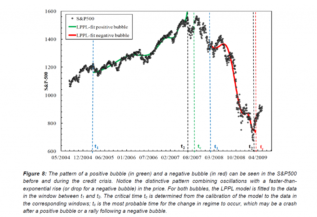
What can we make out of charts such as this, in a recent paper by Sornette and Cauwels?

Sornett and the many researchers collaborating with him over the years are working with a paradigm of an asset bubble as a faster than exponential increase in prices. In an as yet futile effort to extend the olive branch to traditional economists (Sornette is a geophysicist by training), Sornette evokes the “bubbles following from rational expectations meme.” The idea is that it could be rational for an investor to participate in a market that is in the throes of an asset bubble, providing that the investor believes that his gains in the near future adequately compensate for the increased risk of a collapse of prices. This is the “greater fool” theory to a large extent, and I always take delight in pointing out that one of the most intelligent of all human beings – Isaac Newton – was burned by exactly such a situation hundreds of years ago.

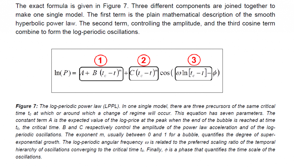
In any case, the mathematics of the Sornette et al approach are organized around the log-periodic power law, expressed in the following equation with the Sornette and Cauwels commentary (click to enlarge).

From a big picture standpoint, the first thing to observe is that there is a parameter t_c in the equation which is the “critical time.”

The whole point of this mathematical apparatus, which derives in part from differential equations and some basic modeling approaches common in physics, is that faster than exponential growth is destined to reach a point at which it basically goes ballistic. That is the critical point. The purpose of forecasting in this context then is to predict when this will be, when will the asset bubble reach its maximum price and then collapse?

And the Sornette framework allows for negative as well as positive price movements according to the dynamics in this equation. So, it is possible, if we can implement this, to predict how far the market will fall after the bubble pops, so to speak, and when it will turn around.

Pretty heady stuff.

The second big picture feature is to note the number of parameters to be estimated in fitting this model to real price data – minimally constants A, B, and C, an exponent m, the angular frequency ω and phase φ, plus the critical time.

For the mathematically inclined, there is a thread of criticism and response, more or less culminating in Clarifications to questions and criticisms on the Johansen–Ledoit–Sornette financial bubble model which used to be available as a PDF download from ETC Zurich.

In brief, the issue is whether the numerical analysis methods fitting the data to the LPPL model arrive at local, instead of global maxima. Obviously, different values for the parameters can lead to wholly different forecasts for the critical time t_c.

To some extent, this issue can be dealt with by running a great number of estimations of the parameters, or by developing collateral metrics for adequacy of the estimates.

But the bottom line is – regardless of the extensive applications of this approach to all manner of asset bubbles internationally and in different markets – the estimation of the parameters seems more in the realm of art, than science, at the present time.

However, it may be that mathematical or computational breakthroughs are possible.

I feel these researchers are “very close.”

In any case, it would be great if there were a package in R or the like to gin up these estimates of the critical time, applying the log-periodic power law.

Then we could figure out “how low it can go.’

And, a final note to this post – it is ironic that as I write and post this, the stock markets have recovered from their recent swoon and are setting new records. So I guess I just want to be prepared, and am not willing to believe the runup can go on forever.

I’m also interested in methodologies that can keep forecasters usefully at work, during the downswing.