A lot of important economic data only are available in quarterly installments. The US Gross Domestic Product (GDP) is one example.

Other financial series and indexes, such as the Chicago Fed National Activity Index, are available in monthly, or even higher frequencies.

Aggregation is a common tactic in this situation. So monthly data is aggregated to quarterly data, and then mapped against quarterly GDP.

But there are alternatives.

One is what Elena Andreou, Eric Ghysels and Andros Kourtellos call a naïve specification –

With daily (D) and quarterly (Q) data, there typically are a proliferation of parameters to estimate – 66 if you allow 22 trading days per month. Here N^D in the above equation is the number of days in the quarterly period.

The usual workaround is a weighting scheme. Thus, two parameter exponential Almon lag polynomials are identified with MIDAS, or Mixed Data Sampling.

However, other researchers note that with the monthly and quarterly data, direct estimation of expressions such as the one above (with X^M instead of X^D ) is more feasible.

The example presented here shows that such models can achieve dramatic gains in accuracy.

Quarterly and Monthly Data Example

Let’s consider forecasting releases of the US nominal Gross Domestic Product by the Bureau of Economic Analysis.

From the BEA’s 2014 News Release Schedule for the National Economic Accounts, one can see that advance estimates of GDP occur a minimum of one month after the end of the quarter being reported. So, for example, the advance estimate for the Third Quarter was released October 30 of this year.

This means the earliest quarter updates on US GDP become available fully a month after the end of the quarter in question.

The Chicago Fed National Activity Index (CFNAI), a monthly guage of overall economic activity, is released three weeks after the month being measured.

So, by the time the preliminary GDP for the latest quarter (analyzed or measured) is released, as many as four CFNAI recent monthly indexes are available, three of which pertain to the months constituting this latest measured quarter.

Accordingly, I set up an equation with a lagged term for GDP growth and fifteen terms or values for CFNAImonthly indexes. For each case, I regress a value for GDP growth for quarter t onto GDP growth for quarter t-1 and values for all the monthly CFNAI indices for quarter t, except for the most recent or last month, and twelve other values for the CFNAI index for the three quarters preceding the final quarter to be estimated – quarter t-1, quarter t-2, and quarter t-3.

One of the keys to this data structure is that the monthly CFNAI values do not “stack,” as it were. Instead the most recent lagged CFNAI value for a case always jumps by three months. So, for the 3rd quarter GDP in, say, 2006, the CFNAI value starts with the value for August 2006 and tracks back 14 values to July 2005. Then for the 4th quarter of 2006, the CFNAI values start with November 2006, and so forth.

This somewhat intricate description supports the idea that we are estimating current quarter GDP just at the end of the current quarter before the preliminary measurements are released.

Data and Estimation

I compile BEA quarterly data for nominal US GDP dating from the first Quarter of 1981 or 1981:1 to the 4^th Quarter of 2011. I also download monthly data from the Chicago Fed National Activity Index from October 1979 to December 2011.

For my dependent or target variable, I calculate year-over-year GDP growth rates by quarter, from the BEA data.

I estimate an equation, as illustrated initially in this post, by ordinary least squares (OLS). For quarters, I use the sample period 1981:2 to 2006:4. The monthly data start earlier to assure enough lagged terms for the CFNAI index, and run from 1979:10 to 2006:12.

Results

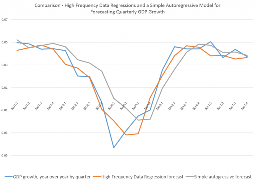
The results are fairly impressive. The regression equation estimated over quarterly and monthly data to the end of 2006 performs much better than a simple first order autocorrelation during the tremendous dip in growth characterizing the Great Recession. In general, even after stabilization of GDP growth in 2010 and 2011, the high frequency data regression produces better out-of-sample forecasts.

Here is a graph comparing the out-of-sample forecast accuracy of the high frequency regression and a simple first order autocorrelation relationship.

What’s especially interesting is that the high frequency data regression does a good job of capturing the drop in GDP and the movement at the turning point in 2009 – the depth of the Great Recession.

I throw this chart up as a proof-of-concept. More detailed methods, using a specially-constructed Chicago Fed index, are described in a paper in the Journal of Economic Perspectives.