Category Archives: cycles

Random Cycles

In 1927, the Russian statistician Eugen Slutsky wrote a classic article called ‘The summation of random causes as the source of cyclic processes,’ a short summary of which is provided by Barnett

If the variables that were taken to represent business cycles were moving averages of past determining quantities that were not serially correlated – either real-world moving averages or artificially generated moving averages – then the variables of interest would become serially correlated, and this process would produce a periodicity approaching that of sine waves

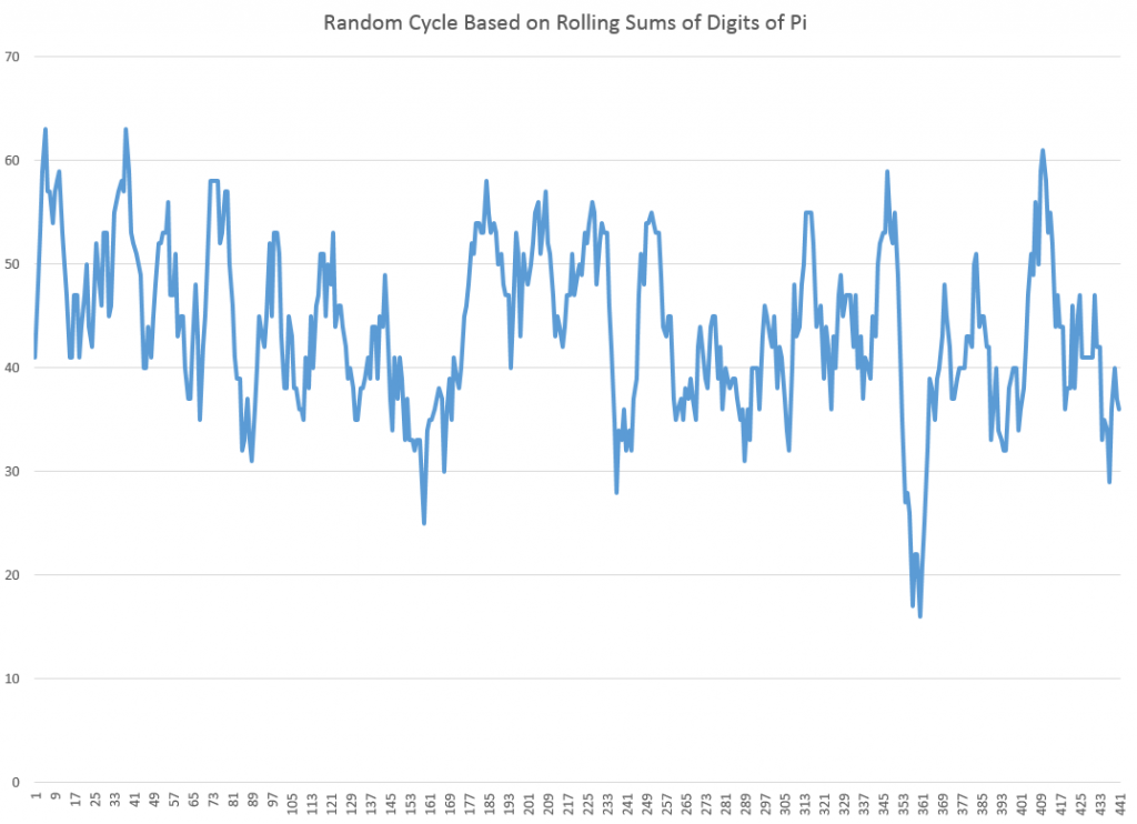
It’s possible to illustrate this phenomena with rolling sums of the digits of pi (π). The following chart illustrates the wave-like result of charting rolling sums of ten consecutive digits of pi.

picycle

So to be explicit, I downloaded the first 450 digits of pi, took them apart, and then graphed the first 440 rolling sums.

The wave-like pattern Illustrates a random cycle.

Forecasting Random Cycles

If we consider this as a time series, each element xk is the following sum,

xk = dk+dk-1+..+dk-10

where dj is the jth digit in the decimal expansion of pi to the right of the initial value of 3.

Now, apparently, it is not proven that the digits of pi are truly random, although one can show that, so far as we can compute, these digits are described by a uniform distribution.

As far as we know, the probability that the next digit will be any digit from 0 to 9 is 1/10=0.1

So as one moves through the digits of pi, generating rolling sums, each new sum means the addition of a new digit, which is unknown and can only be predicted up to its probability. And, at the same time, a digit at the beginning of the preceding sum drops away in the new sum.

Note also that we can always deduce what the series of original digits is, given a series of these rolling sums up to some point.

So the issue is whether the new digit added to the next sum is greater than, equal to, or less than the leading digit of the current sum – which is where we now stand in this sort of analysis. This determines whether the next rolling sum will be greater than, equal to, or less than the current sum.

Here’s where the forecasts can be produced. If the rolling sum is large enough, approaching or equal to 90, there is a high probability that the next rolling sum will be lower, leading to this wave-like pattern. Conversely, if the rolling sum is near zero, the chances are the subsequent sum will be larger. And all this arm-waving can be complemented by exact probabilistic calculations.

Some Ultimate Thoughts

It’s interesting we are really dealing here with a random cycle. That’s proven by the fact that, at any time, the series could go flat-line or trace out some other kind of weird movement.

Thus, the quasi-periodic aspect can be violated for as many periods as you might choose, if one arrives at a run of the same digit in the expansion of pi.

This reminds me of something George Gamow wrote in one of his popular books, where he discusses thermodynamics and the random movement of atoms and molecules in the air of a room. Gamow observes it is entirely possible all the air by chance will congregate in one corner, leaving a vacuum elsewhere. Of course, this is highly improbable.

The only difference would be that there are a finite number of atoms and molecules in the air of any room, but, presumably, an infinite number of digits in the expansion of pi.

The morale of the story is, in any case, to be cautious in imposing a fixed cycle on this type of series.

The Consumer Durable Inventory Cycle – Canary in the Coal Mine?

I’m continuing this week with posts about cycles and, inevitably, need to address one very popular method of extracting cycles from time series data – the Hodrick-Prescott (HP) filter.

Recently, I’ve been exploring inventory cycles, hoping to post something coherent.

I think I hit paydirt, as they say in gold mining circles.

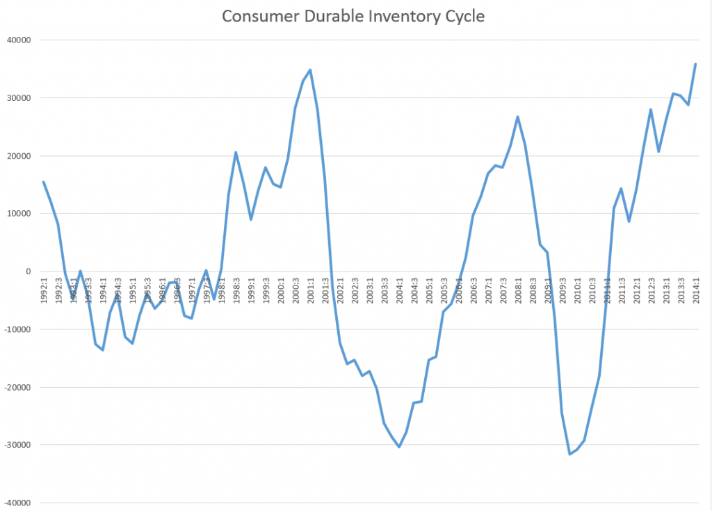
Here is the cycle component extracted from consumer durable inventories (not seasonally adjusted) from the Census manufacturing with a Hodrick-Prescott filter. I use a Matlab implementation here called hpfilter.

CDcycle

In terms of mechanics, the HP filter extracts the trend and cyclical component from a time series by minimizing an expression, as described by Wikipedia –

HPexp

What’s particularly interesting to me is that the peak of the two cycles in the diagram are spot-on the points at which the business cycle goes into recession – in 2001 and 2008.

Not only that, but the current consumer durable inventory cycle is credibly peaking right now and, based on these patterns, should go into a downward movement soon.

Of course, amplitudes of these cycles are a little iffy.

But the existence of a consumer durable cycle configured along these lines is consistent with the literature on inventory cycles, which emphasizes stockout-avoidance and relatively long pro-cyclical swings in inventories.

Semiconductor Cycles

I’ve been exploring cycles in the semiconductor, computer and IT industries generally for quite some time.

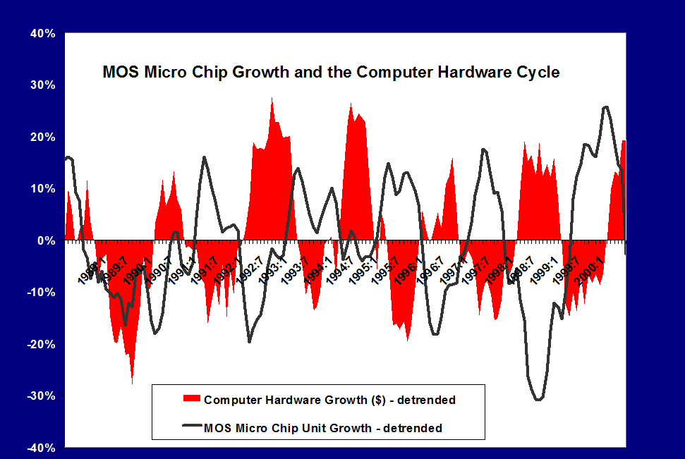
Here is an exhibit I prepared in 2000 for a magazine serving the printed circuit board industry.

semicycle

The data come from two sources – the Semiconductor Industry Association (SIA) World Semiconductor Trade Statistics database and the Census Bureau manufacturing series for computer equipment.

This sort of analytics spawned a spate of academic research, beginning more or less with the work of Tan and Mathews in Australia.

One of my favorites is a working paper released by DRUID – the Danish Research Unit for Industrial Dynamics called Cyclical Dynamics in Three Industries. Tan and Mathews consider cycles in semiconductors, computers, and what they call the flat panel display industry. They start with quoting “industry experts” and, specifically, some of my work with Economic Data Resources on the computer (PC) cycle. These researchers went on to publish in the Journal of Business Research and Technological Forecasting and Social Change in 2010. A year later in 2011, Tan published an interesting article on the sequencing of cyclical dynamics in semiconductors.

Essentially, the appearance of cycles and what I have called quasi-cycles or pseudo-cycles in the semiconductor industry and other IT categories, like computers, result from the interplay of innovation, investment, and pricing. In semiconductors, for example, Moore’s law – which everyone always predicts will fail at some imminent future point – indicates that continuing miniaturization will lead to periodic reductions in the cost of information processing. At some point in the 1980’s, this cadence was firmly established by introductions of new microprocessors by Intel roughly every 18 months. The enhanced speed and capacity of these microprocessors – the “central nervous system” of the computer – was complemented by continuing software upgrades, and, of course, by the movement to graphical interfaces with Windows and the succession of Windows releases.

Back along the supply chain, semiconductor fabs were retooling periodically to produce chips with more and more transitors per volume of silicon. These fabs were, simply put, fabulously expensive and the investment dynamics factors into pricing in semiconductors. There were famous gluts, for example, of memory chips in 1996, and overall the whole IT industry led the recession of 2001 with massive inventory overhang, resulting from double booking and the infamous Y2K scare.

Statistical Modeling of IT Cycles

A number of papers, summarized in Aubrey deploy VAR (vector autoregression) models to capture leading indicators of global semiconductor sales. A variant of these is the Bayesian VAR or BVAR model. Basically, VAR models sort of blindly specify all possible lags for all possible variables in a system of autoregressive models. Of course, some cutoff point has to be established, and the variables to be included in the VAR system have to be selected by one means or another. A BVAR simply reduces the number of possibilities by imposing, for example, sign constraints on the resulting coefficients, or, more ambitiously, employs some type of prior distribution for key variables.

Typical variables included in these models include:

  • WSTS monthly semiconductor shipments (now by subscription only from SIA)
  • Philadelphia semiconductor index (SOX) data
  • US data on various IT shipments, orders, inventories from M3
  • data from SEMI, the association of semiconductor equipment manufacturers

Another tactic is to filter out low and high frequency variability in a semiconductor sales series with something like the Hodrick-Prescott (HP) filter, and then conduct a spectral analysis.

Does the Semiconductor/Computer/IT Cycle Still Exist?

I wonder whether academic research into IT cycles is a case of “redoubling one’s efforts when you lose sight of the goal,” or more specifically, whether new configurations of forces are blurring the formerly fairly cleanly delineated pulses in sales growth for semiconductors, computers, and other IT hardware.

“Hardware” is probably a key here, since there have been big changes since the 1990’s and early years of this brave new century.

For one thing, complementarities between software and hardware upgrades seem to be breaking down. This began in earnest with the development of virtual servers – software which enabled many virtual machines on the same hardware frame, in part because the underlying circuitry was so massively powerful and high capacity now. Significant declines in the growth of sales of these machines followed on wide deployment of this software designed to achieve higher efficiencies of utilization of individual machines.

Another development is cloud computing. Running the data side of things is gradually being taken away from in-house IT departments in companies and moved over to cloud computing services. Of course, critical data for a company is always likely to be maintained in-house, but the need for expanding the number of big desktops with the number of employees is going away – or has indeed gone away.

At the same time, tablets, Apple products and Android machines, created a wave of destructive creation in people’s access to the Internet, and, more and more, for everyday functions like keeping calendars, taking notes, even writing and processing photos.

But note – I am not studding this discussion with numbers as of yet.

I suspect that underneath all this change it should be possible to identify some IT invariants, perhaps in usage categories, which continue to reflect a kind of pulse and cycle of activity.

Some Cycle Basics

A Fourier analysis is one of the first steps in analyzing cycles.

Take sunspots, for example,

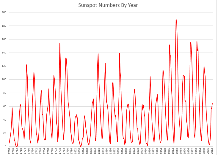
There are extensive historic records on the annual number of sunspots, dating back to 1700. The annual data shown in the following graph dates back to 1700, and is currently maintained by the Royal Belgium Observatory.

sunspots

This series is relatively stationary, although there may be a slight trend if you cut this span of data off a few years before the present.

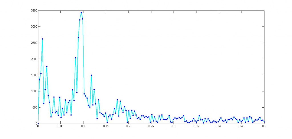
In any case, the kind of thing you get with a Fourier analysis looks like this.

spectralsunspots

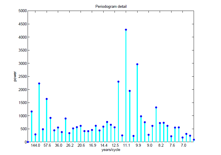
This shows the power or importance of the cycles/year numbers, and maxes out at around 0.09.

These data can be recalibrated into the following chart, which highlights the approximately 11 year major cycle in the sunspot numbers.

sunspotsperiodogramyr

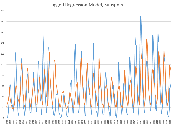
Now it’s possible to build a simple regression model with a lagged explanatory variable to make credible predictions. A lag of eleven years produces the following in-sample and out-of-sample fits. The regression is estimated over data to 1990, and, thus, the years 1991 through 2013 are out-of-sample.

LaggedModel

It’s obvious this sort of forecasting approach is not quite ready for prime-time television, even though it performs OK on several of the out-of-sample years after 1990.

But this exercise does highlight a couple of things.

First, the annual number of sunspots is broadly cyclical in this sense. If you try the same trick with lagged values for the US “business cycle” the results will be radically worse. At least with the sunspot data, most of the fluctuations have timing that is correctly predicted, both in-sample (1990 and before) and out-of-sample (1991-2013).

Secondly, there are stochastic elements to this solar activity cycle. The variation in amplitude is dramatic, and, indeed, the latest numbers coming in on sunspot activity are moving to much lower levels, even though the cycle is supposedly at its peak.

I’ve reviewed several papers on predicting the sunspot cycle. There are models which are more profoundly inspired by the possible physics involved – dynamo dynamics for example. But for my money there are basic models which, on a one-year-ahead basis, do a credible job. More on this forthcoming.