I get excited that principal components offer one solution to the problem of the curse of dimensionality – having fewer observations on the target variable to be predicted, than there are potential drivers or explanatory variables.
It seems we may have to revise the idea that simpler models typically outperform more complex models.
Principal component (PC) regression has seen a renaissance since 2000, in part because of the work of James Stock and Mark Watson (see also) and Bai in macroeconomic forecasting (and also because of applications in image processing and text recognition).
Let me offer some PC basics and explore an example of PC regression and forecasting in the context of macroeconomics with a famous database.
Dynamic Factor Models in Macroeconomics
Stock and Watson have a white paper, updated several times, in PDF format at this link
stock watson generalized shrinkage June _2012.pdf
They write in the June 2012 update,
We find that, for most macroeconomic time series, among linear estimators the DFM forecasts make efficient use of the information in the many predictors by using only a small number of estimated factors. These series include measures of real economic activity and some other central macroeconomic series, including some interest rates and monetary variables. For these series, the shrinkage methods with estimated parameters fail to provide mean squared error improvements over the DFM. For a small number of series, the shrinkage forecasts improve upon DFM forecasts, at least at some horizons and by some measures, and for these few series, the DFM might not be an adequate approximation. Finally, none of the methods considered here help much for series that are notoriously difficult to forecast, such as exchange rates, stock prices, or price inflation.
Here DFM refers to dynamic factor models, essentially principal components models which utilize PC’s for lagged data.
What’s a Principal Component?
Essentially, you can take any bundle of data and compute the principal components. If you mean-center and (in most cases) standardize the data, the principal components divide up the variance of this data, based on the size of their associated eigenvalues. The associated eigenvectors can be used to transform the data into an equivalent and same size set of orthogonal vectors. Really, the principal components operate to change the basis of the data, transforming it into an equivalent representation, but one in which all the variables have zero correlation with each other.
The Wikipaedia article on principal components is useful, but there is no getting around the fact that principal components can only really be understood with matrix algebra.
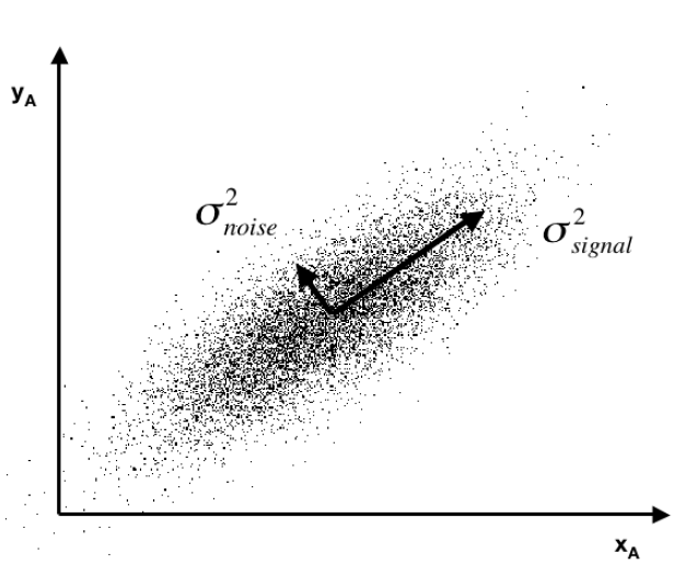
Often you see a diagram, such as the one below, showing a cloud of points distributed around a line passing through the origin of a coordinate system, but at an acute angle to those coordinates.
This illustrates dimensionality reduction with principal components. If we express all these points in terms of this rotated set of coordinates, one of these coordinates – the signal – captures most of the variation in the data. Projections of the datapoints onto the second principal component, therefore, account for much less variance.
Principal component regression characteristically specifies only the first few principal components in the regression equation, knowing that, typically, these explain the largest portion of the variance in the data.
It’s also noteworthy that some researchers are talking about “targeted” principal components. So the first few principal components account for the largest, the next largest, and so on amount of variance in the data. However, the “data” in this context does not include the information we have on the target variable. Targeted principal components therefore involves first developing the simple correlations between the target variable and all the potential predictors, then ordering these potential predictors from highest to lowest correlation. Then, by one means or another, you establish a cutoff, below which you exclude weak potential predictors from the data matrix you use to compute the principal components. Interesting approach which makes sense. Testing it with a variety of examples seems in order.
PC Regression and Forecasting – A Macroeconomics Example
I downloaded a trial copy of XLSTAT – an Excel add-in with a well-developed set of principal component procedures. In the past, I’ve used SPSS and SAS on corporate networked systems. Now I am using Matlab and GAUSS for this purpose.
The problem is what does it mean to have a time series of principal components? Over the years, there have been relevant discussions – Jolliffe’s key work, for example, and more recent papers.
The problem with time series, apart from the temporal interdependencies, is that you always are calculating the PC’s over different data, as more data comes in. What does this do to the PC’s or factor scores? Do they evolve gradually? Can you utilize the factor scores from a smaller dataset to predict subsequent values of factor scores estimated over an augmented dataset?
Based on a large macroeconomic dataset I downloaded from Mark Watson’s page, I think the answer can be a qualified “yes” to several of these questions. The Mark Watson dataset contains monthly observations on 106 macroeconomic variables for the period 1950 to 2006.
For the variables not bounded within a band, I calculated year-over-year (yoy) growth rates for each monthly observation. Then, I took first differences again over 12 months. These transformations eliminated trends, which mess up the PC computations (basically, if you calculate PC’s with a set of increasing variables, the first PC will represent a common growth factor, and is almost useless for modeling purposes.) The result of my calculations was to center each series at nearly zero, and to make the variability of each series comparable – so I did not standardize.
Anyway, using XLSTAT and Forecast Pro – I find that the factor scores
(a) Evolve slowly as you add more data.
(b) Factor scores for smaller datasets provide insight into subsequent factor scores one to several months ahead.
(c) Amazingly, turning points of the first principal component, which I have studied fairly intensively, are remarkably predictable.
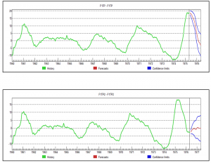
So what are we looking at here (click to enlarge)?
Well, the top chart is the factor score for the first PC, estimated over data to May 1975, with a forecast indicated by the red line at the right of the graph. This forecast produces values which are very close to the factor score values for data estimated to May 1976 – where both datasets begin in 1960. Not only that, but we have here an example of prediction of a turning point bigtime.
Of course this is the magic of Box-Jenkins, since, this factor score series is best estimated, according to Forecast Pro, with an ARIMA model.
I’m encouraged by this exercise to think that it may be possible to go beyond the lagged variable specification in many of these DFM’s to a contemporaneous specification, where the target variable forecasts are based on extrapolations of the relevant PC’s.
In any case, for applied business modeling, if we got something like a medical device new order series (suitably processed data) linked with these macro factor scores, it could be interesting – and we might get something that is not accessible with ordinary methods of exponential smoothing.
Underlying Theory of PC’s
Finally, I don’t think it is possible to do much better than to watch Andrew Ng at Stanford in Lectures 14 and 15. I recommend skipping to 17:09 – seventeen minutes and nine seconds – into Lecture 14, where Ng begins the exposition of principal components. He winds up this Lecture with a fascinating illustration of high dimensionality principal component analysis applied to recognizing or categorizing faces in photographs at the end of this lecture. Lecture 15 also is very useful – especially as it highlights the role of the Singular Value Decomposition (SVD) in actually calculating principal components.
Lecture 14
http://www.youtube.com/watch?v=ey2PE5xi9-A
Lecture 15

