There’s a straight-forward way to understand the value and potential significance of quantile regression – consider the hurricane data referenced in James Elsner’s blog Hurricane & Tornado Climate.
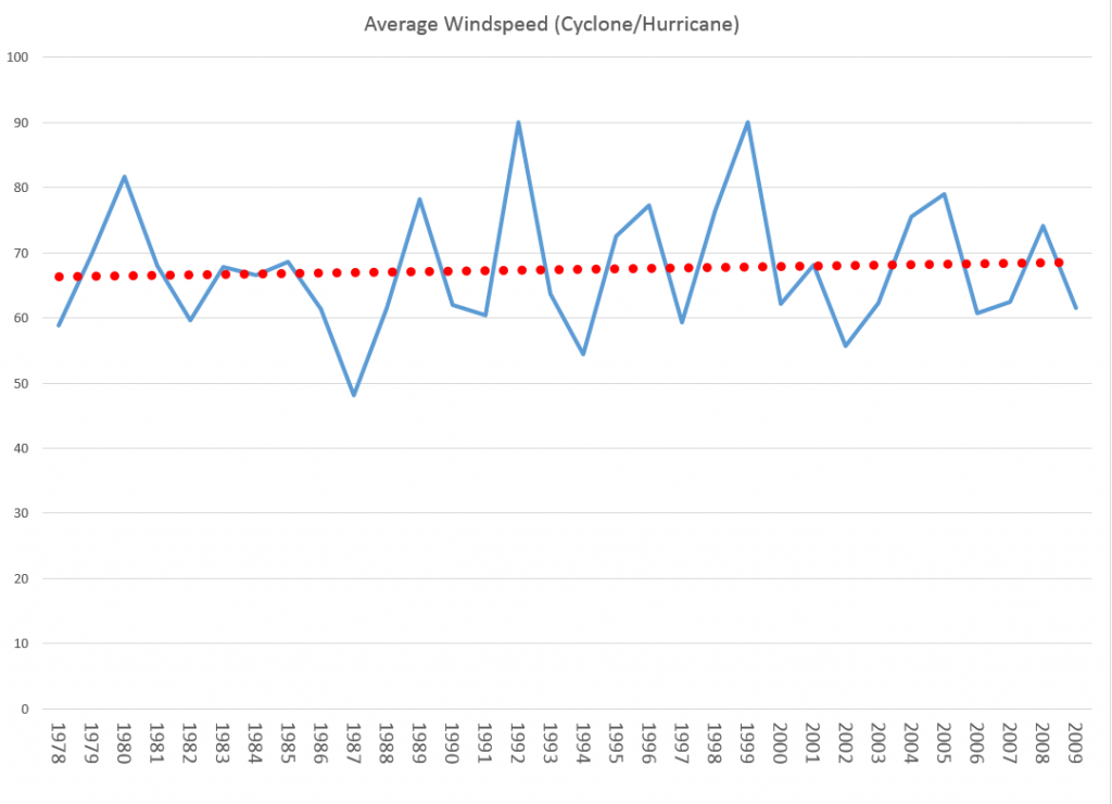
Here is a plot of average windspeed of hurricanes in the Atlantic and Gulf Coast since satellite observations began after 1977.
Based on averages, the linear trend line increases about 2 miles per hour over this approximately 30 year period.
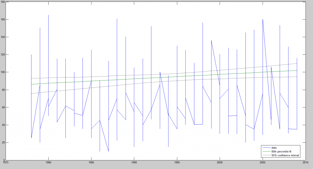
An 80th percentile quantile regression trend line, on the other hand, with this data indicates that the trend in the more violent hurricanes shows an about 15 mph increase over this same period.
In other words, if we look at the hurricanes which are in the 80th percentile or more, there is a much stronger trend in maximum wind speeds, than in the average for all US-related hurricanes in this period.
A quantile q, 0<q<1, splits the data into proportions q below and 1-q above. The most familiar quantile, thus, may be the 50th percentile which is the quantile which splits the data at the median – 50 percent below and 50 percent above.
Quantile regression (QR) was developed, in its modern incarnation by Koenker and Basset in 1978. QR is less influenced by non-normal errors and outliers, and provides a richer characterization of the data.
Thus, QR encourages considering the impact of a covariate on the entire distribution of y, not just is conditional mean.
Roger Koenker and Kevin F. Hallock’s Quantile Regression in the Journal of Economic Perspectives 2001 is a standard reference.
We say that a student scores at the tth quantile of a standardized exam if he performs better than the proportion t of the reference group of students and worse than the proportion (1–t). Thus, half of students perform better than the median student and half perform worse. Similarly, the quartiles divide the population into four segments with equal proportions of the reference population in each segment. The quintiles divide the population into five parts; the deciles into ten parts. The quantiles, or percentiles, or occasionally fractiles, refer to the general case.
Just as we can define the sample mean as the solution to the problem of minimizing a sum of squared residuals, we can define the median as the solution to the problem of minimizing a sum of absolute residuals.
Ordinary least squares (OLS) regression minimizes the sum of squared errors of observations minus estimates. This minimization leads to explicit equations for regression parameters, given standard assumptions.
Quantile regression, on the other hand, minimizes weighted sums of absolute deviations of observations on a quantile minus estimates. This minimization problem is solved by the simplex method of linear programming, rather than differential calculus. The solution is robust to departures from normality of the error process and outliers.
Koenker’s webpage is a valuable resource with directions for available software to estimate QR. I utilized Mathworks Matlab for my estimate of a QR with the hurricane data, along with a supplemental program for quantreg(.) I downloaded from their site.
Here are a couple of short, helpful videos from Econometrics Academy.
Featured image from http://www.huffingtonpost.com/2012/10/29/hurricane-sandy-apps-storm-tracker-weather-channel-red-cross_n_2039433.html


