Volatility of stock market returns is more predictable, in several senses, than stock market returns themselves.

Generally, if p_t is the price of a stock at time t, stock market returns often are defined as ln(p_t)-ln(p_t-1). Volatility can be the absolute value of these returns, or as their square. Thus, hourly, daily, monthly or other returns can be positive or negative, while volatility is always positive.

Masset highlights several stylized facts about volatility in a recent paper –

• Volatility is not constant and tends to cluster through time. Observing a large (small) return today (whatever its sign) is a good precursor of large (small) returns in the coming days.

• Changes in volatility typically have a very long-lasting impact on its subsequent evolution. We say that volatility has a long memory.

• The probability of observing an extreme event (either a dramatic downturn or an enthusiastic takeoff) is way larger than what is hypothesized by common data generating processes. The returns distribution has fat tails.

• Such a shock also has a significant impact on subsequent returns. Like in an earthquake, we typically observe aftershocks during a number of trading days after the main shock has taken place.

• The amplitude of returns displays an intriguing relation with the returns themselves: when prices go down – volatility increases; when prices go up – volatility decreases but to a lesser extent. This is known as the leverage effect … or the asymmetric volatility phenomenon.

• Recently, some researchers have noticed that there were also some significant differences in terms of information content among volatility estimates computed at various frequencies. Changes in low-frequency volatility have more impact on subsequent high-frequency volatility than the opposite. This is due to the heterogeneous nature of market participants, some having short-, medium- or long-term investment horizons, but all being influenced by long-term moves on the markets…
• Furthermore, … the intensity of this relation between long and short time horizons depends on the level of volatility at long horizons: when volatility at a long time horizon is low, this typically leads to low volatility at short horizons too. The reverse is however not always true…

Masset extends and deepens this type of result for bull and bear markets and developed/emerging markets. Generally, emerging markets display higher volatility with some differences in third and higher moments.

A key reference is Rami Cont’s Empirical properties of asset returns: stylized facts and statistical issues which provides this list of features of stock market returns, some of which directly relate to volatility. This is one of the most widely-cited articles in the financial literature:

1. Absence of autocorrelations: (linear) autocorrelations of asset returns are often insignificant, except for very small intraday time scales (~20 minutes) for which microstructure effects come into play.
2. Heavy tails: the (unconditional) distribution of returns seems to display a power-law or Pareto-like tail, with a tail index which is finite, higher than two and less than five for most data sets studied. In particular this excludes stable laws with infinite variance and the normal distribution. However the precise form of the tails is difficult to determine.
3. Gain/loss asymmetry: one observes large drawdowns in stock prices and stock index values but not equally large upward movements.
4. Aggregational Gaussianity: as one increases the time scale t over which returns are calculated, their distribution looks more and more like a normal distribution. In particular, the shape of the distribution is not the same at different time scales.
5. Intermittency: returns display, at any time scale, a high degree of variability. This is quantified by the presence of irregular bursts in time series of a wide variety of volatility estimators.
6. Volatility clustering: different measures of volatility display a positive autocorrelation over several days, which quantifies the fact that high-volatility events tend to cluster in time.
7. Conditional heavy tails: even after correcting returns for volatility clustering (e.g. via GARCH-type models), the residual time series still exhibit heavy tails. However, the tails are less heavy than in the unconditional distribution of returns.
8. Slow decay of autocorrelation in absolute returns: the autocorrelation function of absolute returns decays slowly as a function of the time lag, roughly as a power law with an exponent β ∈ [0.2, 0.4]. This is sometimes interpreted as a sign of long-range dependence.
9. Leverage effect: most measures of volatility of an asset are negatively correlated with the returns of that asset.
10. Volume/volatility correlation: trading volume is correlated with all measures of volatility.
11. Asymmetry in time scales: coarse-grained measures of volatility predict fine-scale volatility better than the other way round.

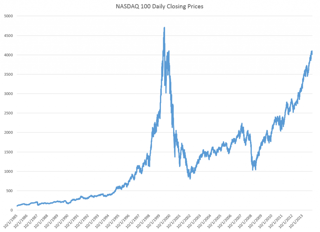
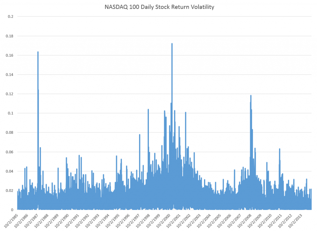
Just to position the discussion, here are graphs of the NASDAQ 100 daily closing prices and the volatility of daily returns, since October 1, 1985.

The volatility here is calculated as the absolute value of the differences of the logarithms of the daily closing prices.