I think it is about time for another dive into stock market forecasting. The US market is hitting new highs with the usual warnings of excess circulating around. And there are interesting developments in volatility.
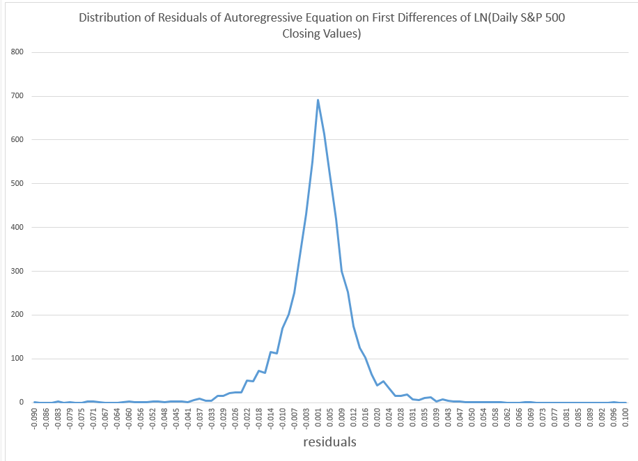
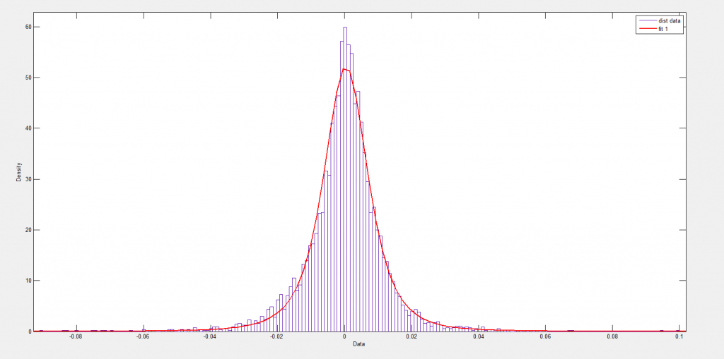
To get things rolling, consider the following distribution of residuals from an autoregressive model on the difference in the natural logarithms of the S&P 500.
This is what I am calling “the distribution of daily stock market returns.” I’ll explain that further in a minute.
Now I’ve seen this distribution before, and once asked in a post, “what type of distribution is this?”
Now I think I have the answer – it’s a Laplace distribution, sometimes known as the double exponential distribution.
Since this might be important, let me explain the motivation and derivation of these residuals, and then consider some implications.
Derivation of the Residuals
First, why not just do a histogram of the first differences of daily returns to identify the underlying distribution? After all, people say movement of stock market indexes are a random walk.
OK, well you could do that, and the resulting distribution would also look “Laplacian” with a pointy peak and relative symmetry. However, I am bothered in developing this by the fact that these first differences show significant, even systematic, autocorrelation.
I’m influenced here by the idea that you always want to try to graph independent draws from a distribution to explore the type of distribution.
OK, now to details of my method.
The data are based on daily closing values for the S&P 500 index from December 4, 1989 to February 7, 2014.
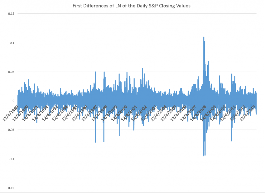
I took the natural log of these closing values and then took first differences – subtracting the previous trading day’s closing value from the current day’s closing value. This means that these numbers encode the critical part of the daily returns, which are calculated as day-over-day percent changes. Thus, the difference of natural logs is in fact a ratio of the original numbers – what you might look at as the key part of the percent change from one trading day to the next.
So I generate a conventional series of first differences of the natural log of this nonstationary time series. This transforms the original nonstationary series to a one that basically fluctuates around a level – essentially zero. Furthermore, the log transform tends to reduce the swings in the variability of the series, although significant variability remains.
Removing Serial Correlation
The series graphed above exhibits first order serial correlation. It also exhibits second order serial correlation, or correlation between values at a lag of 2.
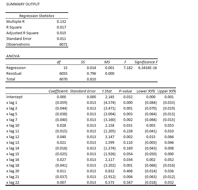
Based on the correlations for the first 24 lags, I put together this regression equation. Of course, the “x’s” refer to time dated first differences of the natural log of the S&P daily closing values.
Note that most of the t-statistics pass our little test of significance (which I think is predicted to an extent on the error process belonging to certain distributions..but). The coefficient of determination or R2 is miniscule – at 0.017. This autoregressive equation thus explains only about 2 percent of the variation in this differenced log daily closing values series.
Now one of the things I plan to address is how, indeed, that faint predictive power can exert significant influence on earnings from stock trading, given trading rules.
But let me leave that whole area – how you make money with such a relationship – to a later discussion, since I’ve touched on this before.
Instead, let me just observe that if you subtract the predicted values from this regression from the actuals trading day by trading day, you get the data for the pointy, highly symmetric distribution of residuals.
Furthermore, these residuals do not exhibit first or second, or higher, autocorrelation, so far as I am able to determine.
This means we have separated out algorithmic components of this series from random components that are not serially correlated.
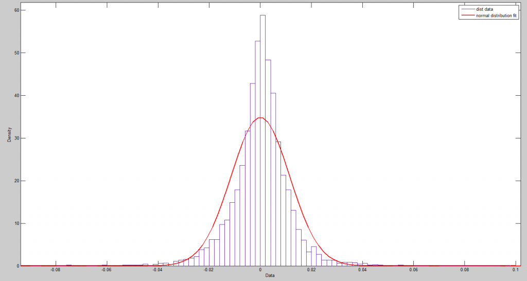
So you might jump to the conclusion that these residuals are then white noise, and I think many time series modelers have gotten to this point, simply assuming they are dealing with Gaussian white noise.
Nothing could be further from the truth, as the following Matlab fit of a normal distribution to some fairly crude bins for these numbers.
A Student-t distribution does better, as the following chart shows.
But the t-distribution still misses the pointed peak.
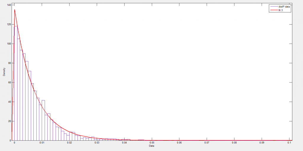
The Laplace distribution is also called the double exponential, since it can be considered to be a composite of exponentials on the right and to the left of the mean – symmetric but mirror images of each other.
The following chart shows how this works over the positive residuals.
Now, of course, there are likelihood ratios and those sorts of metrics, and I am busy putting together a comparison between the t-distribution fit and Laplace distribution fit.
There is a connection between the Laplace distribution and power laws, too, and I note considerable literature on this distribution in finance and commodities.
I think I have answered the question I put out some time back, though, and, of course, it raises other questions in its wake.

