Tag Archives: financial forecasts

The Apostle of Negative Interest Rates

Miles Kimball is a Professor at the University of Michigan, and a vocal and prolific proponent of negative interest rates. His Confessions of a Supply-Side Liberal is peppered with posts on the benefits of negative interest rates.

March 2 Even Central Bankers Need Lessons on the Transmission Mechanism for Negative Interest Rates, after words of adoration, takes the Governor of the Bank of England (Mark Carney) to task. Carney’s problem? Carney wrote recently that unless regular households face negative interest rates in their deposit accounts.. negative interest rates only work through the exchange rate channel, which is zero-sum from a global point of view.

Kimball’s argument is a little esoteric, but promotes three ideas.

First, negative interest rates central bank charge member banks on reserves should be passed onto commercial and consumer customers with larger accounts – perhaps with an exemption for smaller checking and savings accounts with, say, less than $1000.

Second, moving toward electronic money in all transactions makes administration of negative interest rates easier and more effective. In that regard, it may be necessary to tax transactions conducted in paper money, if a negative interest rate regime is in force.

Third, impacts on bank profits can be mitigated by providing subsidies to banks in the event the central bank moved into negative interest rate territory.

Fundamentally, Kimball’s view is that.. monetary policy–and full-scale negative interest rate policy in particular–is the primary answer to the problem of insufficient aggregate demand. No need to set inflation targets above zero in order to get the economy moving. Just implement sufficiently negative interest rates and things will rebound quickly.

Kimball’s vulnerability is high mathematical excellence coupled with a casual attitude toward details of actual economic institutions and arrangements.

For example, in his Carney post,  Kimball offers this rather tortured prose under the heading -“Why Wealth Effects Would Be Zero With a Representative Household” –

It is worth clarifying why the wealth effects from interest rate changes would have to be zero if everyone were identical [sic, emphasis mine]. In aggregate, the material balance condition ensures that flow of payments from human and physical capital have not only the same present value but the same time path and stochastic pattern as consumption. Thus–apart from any expansion of the production of the economy as a whole as a result of the change in monetary policy–any effect of interest rate changes on the present value of society’s assets overall is cancelled out by the effect of interest rate changes on the present value of the planned path and pattern of consumption. Of course, what is actually done will be affected by the change in interest rates, but the envelope theorem says that the wealth effects can be calculated based on flow of payments and consumption flows that were planned initially.

That’s in case you worried a regime of -2 percent negative interest rates – which Kimball endorses to bring a speedy end to economic stagnation – could collapse the life insurance industry or wipe out pension funds.

And this paragraph is troubling from another standpoint, since Kimball believes negative interest rates or “monetary policy” can trigger “expansion of the production of the economy as a whole.” So what about those wealth effects?

Indeed, later in the Carney post he writes,

..for any central bank willing to go off the paper standard, there is no limit to how low interest rates can go other than the danger of overheating the economy with too strong an economic recovery. If starting from current conditions, any country can maintain interest rates at -7% or lower for two years without overheating its economy, then I am wrong about the power of negative interest rates. But in fact, I think it will not take that much. -2% would do a great deal of good for the eurozone or Japan, and -4% for a year and a half would probably be enough to do the trick of providing more than enough aggregate demand.

At the end of the Carney post, Kimball links to a list of his and other writings on negative interest rates called How and Why to Eliminate the Zero Lower Bound: A Reader’s Guide. Worth bookmarking.

Here’s a YouTube video.

Although not completely fair, I have to say all this reminds me of a widely-quoted passage from Keynes’ General Theory –

“Practical men who believe themselves to be quite exempt from any intellectual influence, are usually the slaves of some defunct economist. Madmen in authority, who hear voices in the air, are distilling their frenzy from some academic scribbler of a few years back”

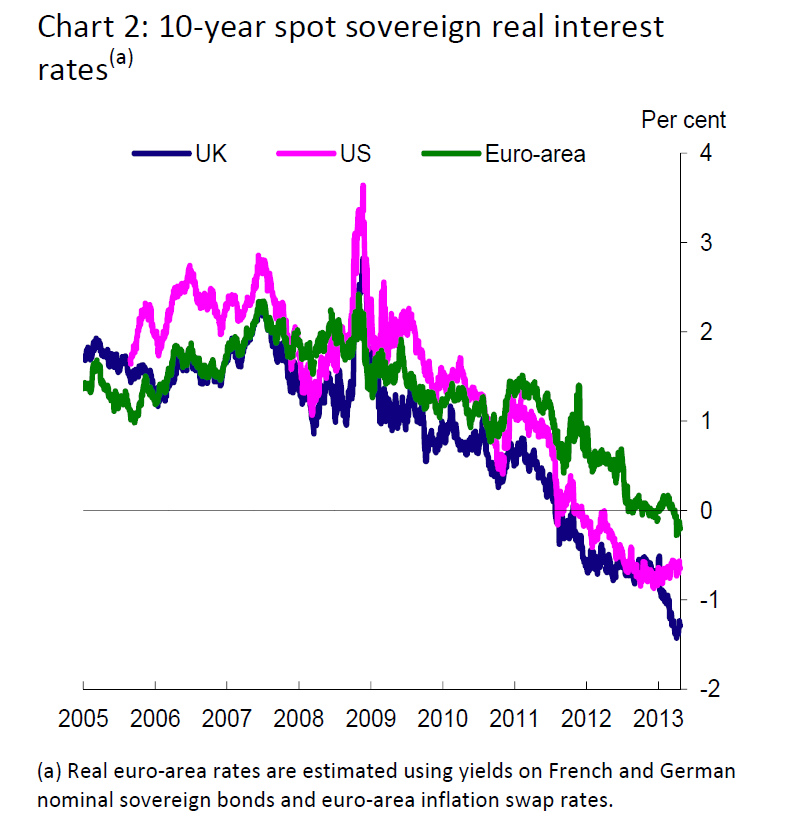
Of course, the policy issue behind the spreading adoption of negative interest rates is that the central banks of the world are, in many countries, at the zero bound already. Thus, unless central banks can move into negative interest rate territory, governments are more or less “out of ammunition” when it comes to combatting the next recession – assuming, of course, that political alignments currently favoring austerity over infrastructure investment and so forth, are still in control.

The problem I have might be posed as one of “complexity theory.”

I myself have spent hours pouring over optimal control models of consumption  and dynamic general equilibrium. This stuff is so rarified and intellectually challenging, really, that it produces a mindset that suggests mastery of Portryagin’s maximum principle in a multi-equation setup means you have something relevant to say about real economic affairs. In fact, this may be doubtful, especially when the linkages between organizations are so complex, especially dynamically.

The problem, indeed, may be institutional but from a different angle. Economics departments in universities have, as their main consumer, business school students. So economists have to offer something different.

One would hope machine learning, Big Data, and the new predictive analytics, framed along the lines outlined by Hal Varian and others, could provide an alternative paradigm for economists – possibly rescuing them from reliance on adjusting one number in equations that are stripped of the real, concrete details of economic linkages.

Negative Interest Rates

What are we to make of negative interest rates?

Burton Malkiel (Princeton) writes in the Library of Economics and Liberty that The rate of interest measures the percentage reward a lender receives for deferring the consumption of resources until a future date. Correspondingly, it measures the price a borrower pays to have resources now.

So, in a topsy-turvy world, negative interest rates might measure the penalty a lender receives for delaying consumption of resources to some future date from a more near-term date, or from now.

This is more or less the idea of this unconventional monetary policy, now taking hold in the environs of the European and Japanese Central Banks, and possibly spreading sometime soon to your local financial institution. Thus, one of the strange features of business behavior since the Great Recession of 2008-2009 has been the hoarding of cash either in the form of retained corporate earnings or excess bank reserves.

So, in practical terms, a negative interest rate flips the relation between depositors and banks.

With negative interest rates, instead of receiving money on deposits, depositors must pay regular sums, based on the size of their deposits, to keep their money with the bank.

“If rates go negative, consumer deposit rates go to zero and PNC would charge fees on accounts.”

The Bank of Japan, the European Central Bank and several smaller European authorities have ventured into this once-uncharted territory recently.

Bloomberg QuickTake on negative interest rates

The Bank of Japan surprised markets Jan. 29 by adopting a negative interest-rate strategy. The move came 1 1/2 years after the European Central Bank became the first major central bank to venture below zero. With the fallout limited so far, policy makers are more willing to accept sub-zero rates. The ECB cut a key rate further into negative territory Dec. 3, even though President Mario Draghi earlier said it had hit the “lower bound.” It now charges banks 0.3 percent to hold their cash overnight. Sweden also has negative rates, Denmark used them to protect its currency’s peg to the euro and Switzerland moved its deposit rate below zero for the first time since the 1970s. Since central banks provide a benchmark for all borrowing costs, negative rates spread to a range of fixed-income securities. By the end of 2015, about a third of the debt issued by euro zone governments had negative yields. That means investors holding to maturity won’t get all their money back. Banks have been reluctant to pass on negative rates for fear of losing customers, though Julius Baer began to charge large depositors.

These developments have triggered significant criticism and concern in the financial community.

Japan’s Negative Interest Rates Are Even Crazier Than They Sound

The Japanese government got paid to borrow money for a decade for the first time, selling 2.2 trillion yen ($19.5 billion) of the debt at an average yield of minus 0.024 percent on Tuesday…

The central bank buys as much as 12 trillion yen of the nation’s government debt a month…

Life insurance companies, for instance, take in premiums today and invest them to be able to cover their obligations when policyholders eventually die. They price their policies on the assumption of a mid-single-digit positive return on their bond portfolios. Turn that return negative and all of a sudden the world’s life insurers are either unprofitable or insolvent. And that’s a big industry.

Pension funds, meanwhile, operate the same way, taking in and investing contributions against future obligations. Many US pension plans are already borderline broke, and in a NIRP environment they’ll suffer a mass extinction. Again, big industry, many employees, huge potential impact on both Wall Street and Main Street.

It has to be noted, however, that real (or inflation-adjusted) interest rates have gone below zero already for certain asset classes. Thus, a highlight of the Bank of England Study on negative interest rates circa 2013 is this chart, showing the emergence of negative real interest rates.

NegRealIR

Are these developments the canary in the mine?

We really need some theoretical analysis from the economics community – perspectives that encompass developments like the advent of China as a major player in world markets and patterns of debt expansion and servicing in the older industrial nations.

An Update on Bitcoin

Fairly hum-drum days of articles on testing for unit roots in time series led to discovery of an extraordinary new forecasting approach – using the future to predict the present.

Since virtually the only empirical application of the new technique is predicting bubbles in Bitcoin values, I include some of the recent news about Bitcoins at the end of the post.

Noncausal Autoregressive Models

I think you have to describe the forecasting approach recently considered by Lanne and Saikkonen, as well as Hencic, Gouriéroux and others, as “exciting,” even “sexy” in a Saturday Night Live sort of way.

Here is a brief description from a 2015 article in the Econometrics of Risk called Noncausal Autoregressive Model in Application to Bitcoin/USD Exchange Rates

noncausal

I’ve always been a little behind the curve on lag operators, but basically Ψ(L-1) is a function of the standard lagged operators, while Φ(L) is a second function of offsets to future time periods.

To give an example, consider,

yt = k1yt-1+s1yt+1 + et

where subscripts t indicate time period.

In other words, the current value of the variable y is related to its immediately past value, and also to its future value, with an error term e being included.

This is what I mean by the future being used to predict the present.

Ordinarily in forecasting, one would consider such models rather fruitless. After all, you are trying to forecast y for period t+1, so how can you include this variable in the drivers for the forecasting setup?

But the surprising thing is that it is possible to estimate a relationship like this on historic data, and then take the estimated parameters and develop simulations which lead to predictions at the event horizon, of, say, the next period’s value of y.

This is explained in the paragraph following the one cited above –

noncausal2

In other words, because et in equation (1) can have infinite variance, it is definitely not normally distributed, or distributed according to a Gaussian probability distribution.

This is fascinating, since many financial time series are associated with nonGaussian error generating processes – distributions with fat tails that often are platykurtotic.

I recommend the Hencic and Gouriéroux article as a good read, as well as interesting analytics.

The authors proposed that a stationary time series is overlaid by explosive speculative periods, and that something can be abstracted in common from the structure of these speculative excesses.

Mt. Gox, of course, mentioned in this article, was raided in 2013 by Japanese authorities, after losses of more than $465 million from Bitcoin holders.

Now, two years later, the financial industry is showing increasing interest in the underlying Bitcoin technology and Bitcoin prices are on the rise once again.

bitcoin

Anyway, the bottom line is that I really, really like a forecast methodology based on recognition that data come from nonGaussian processes, and am intrigued by the fact that the ability to forecast with noncausal AR models depends on the error process being nonGaussian.

Recent Events in the US Stock Market

The recent drop in US stocks is dramatic, as the steep falloff of the SPY exchange traded fund (ETF) Monday, August 24th– almost the most recent action in the chart – shows.

SPYAUG26

At the same time, this is by no means the steepest drop in closing prices, as the following chart of daily returns highlights.

SPYDailyReturns

TV commentators and others point to China and the prospective liftoff of US short term interest rates, with the Federal Reserve finally raising rates off the zero bound in – it was thought – September.

I have been impressed at the accuracy of Michael Pettis’ predictions in his China Financial Markets. Pettis has warned about a debt bubble in China for two years and consistently makes other correct calls. I have some first-hand experience doing business in China, and plan a longer post of the collapse of Chinese stock markets and the economic slowdown there.

You can imagine, if you will, a sort of global input-output table with a corresponding table of import/export flows. China has gotten a lot bigger since 2008-2009, absorbing significant amounts of the global output of iron and steel, oil, and other commodities.

Also, in 2008-2009 and in the earlier recession of 2001, China led the way to greater spending, buoying the global economy which, otherwise, was in sad shape. That’s not going to happen this time, if a real recession takes hold.

All very scary, but while the latest stuff took place, this is what I was doing.

CliveChair

In other words, I was the father of the groom at a splendid wedding for my younger son at the Pearl Buck estate just outside Philadelphia.

Well, that wonderful thing being done, I plan to return to more frequent posting on BusinessForecastblog.

I also apologize for having the tools to predict the current downturn, at least after developments later last week, and not signaling readers.

But frankly, I’m not sure the extreme value prediction algorithms (EVPA) reliably predict major turning points. In fact, there seem to be outside influences at key junctures. However, once a correction is underway, predictability returns. Thus, the algorithms do more than simply forecast the growth in stock prices. The EVPA also works to predict the extent of downturns.

Here’s a tip. Start watching ratios such as those between  differences between the  opening price in a trading day and the previous day’s high or low price, divided by the previous day’s high or low price, respectively. Very significant predictors of the change in daily highs and lows, and with significance for changes in closing prices, if you bring some data analytics to bear.

Chinese Stock Market Collapse

Chinese stocks are more volatile, in terms of percent swings, than stocks on other global markets, as this Bloomberg chart highlights.

ChinaStockVolatileGlobal

So the implication is maybe that the current bursting of the Chinese stock bubble is not such a big deal for the global economy, or perhaps it can be contained – despite signs of correlations between the Global Stocks and Shanghai Composite series.

Facts and Figures

Panic selling hit the major Chinese exchanges in Shanghai and Shenzeng, spreading now to the Hong Kong exchange.

Trades on most companies are limited or frozen, and major indexes continue to drop, despite support from the Chinese government.

Chinese Trading Suspensions Freeze $1.4 Trillion of Shares Amid Rout

The rout in Chinese shares has erased at least $3.2 trillion in value, or twice the size of India’s entire stock market. The Shenzhen Composite Index has led declines with a 38 percent plunge since its June 12 peak, as margin traders unwound bullish bets.

China: The Stock Market Meltdown Continues

Briefly put, there are few alternatives for saving in China. The formal banking system provides negative returns (low deposit yields, lower than inflation typically). Housing is no longer returning positive capital gains — partly as a consequence of deliberate policy actions to moderate a perceived housing bubble. So, what’s left (given you can’t easily save in overseas assets)? Equities. We have a typical boom-bust phenomenon, amplified by underdeveloped financial markets, opacity in valuations, and uncertainty regarding the government’s intentions (and will-power).

Stock Sell-Off Is Unabated in China (New York Times)

Most of the trades on Chinese exchanges are made by “retail traders,” basically individuals speculating on the market. These individuals often are highly leveraged or operating with borrowed money.

The Chinese markets moved into bubble territory several months back, and when a correction hit and as it accelerated recently, the Chinese government has tried all sorts of stuff, some charted below.

Chinameasures

Public/private funds to buy stocks and slow the fall in their prices have been created, also.

Risks of Contagion

It’s hard for foreign investors to gain access to the Chinese markets, where there are different classes of stocks for Chinese and foreign traders. So, by that light, only a few percent of Chinese stocks are held by foreign interests, and direct linkages between the sharp turn in values in China and elsewhere should be limited.

There may indirect linkages going from the Chinese stock market to the Chinese economy, and then to foreign supplies.

Here’s why the crash in Chinese stocks matters so much to Australia, i.e.  Australian property markets and reduced Chinese demand for iron.

Iron ore demand by China and the drop in Chinese stocks actually seems more related to somewhat independent linkage with the longer term cascade down by Chinese GDP growth, illustrated here (See Ongoing Developments in China).

ChinaGDPgr

But maybe the most dangerous and unpredictable linkage is psychological.

Thus, the Financial Express of India reports Shanghai blues trigger panic selling on Dalal Street, metals feel the heat

Rational Bubbles

A rational bubble exists when investors are willing to pay more for stocks than is justified by the discounted stream of future dividends. If investors evaluate potential gains from increases in the stock price as justifying movement away from the “fundamental value” of the stock – a self-reinforcing process of price increases can take hold, but be consistent with “rational expectations.”

This concept has been around for a while, and can be traced to eminences such as Oliver Blanchard, now Chief Economist for the International Monetary Fund (IMF), and Mark Watson, Professor of Economics at Princeton University – (See Bubbles, Rational Expectations and Financial Markets).

In terms of formal theory, Diba and Grossman offer a sophisticated analysis in The Theory of Rational Bubbles in Stock Prices. They invoke intriguing language such as “explosive conditional expectations” and the like.

Since these papers from the 1980’s, the relative size of the financial sector has ballooned, and valuation of derivatives now dwarfs totals for annual value of production on the planet (See Bank for International Settlements).

And, in the US, we have witnessed two, dramatic stock market bubbles, here using the phrase in a more popular “plain-as-the-hand-in-front-of-your-face” sense.

SP500

Following through the metaphor, bursting of the bubble leaves financial plans in shambles, and, from the evidence of parts of Europe at least, can cause significant immiseration of large segments of the population.

It would seem reasonable, therefore, to institute some types of controls, as a bubble was emerging. Perhaps an increase in financial transactions taxes, or some other tactic to cause investors to hold stocks for longer periods.

The question, then, is whether it is possible to “test” for a rational bubble pre-emptively or before-the-fact.

So I have been interested recently to come on more recent analysis of so-called rational bubbles, applying advanced statistical techniques.

I offer some notes and links to download the relevant papers.

These include ground-breaking work by Craine in a working paper Rational Bubbles: A Test.

Then, there are two studies focusing on US stock prices (I include extracts below in italics):

Testing for a Rational Bubble Under Long Memory

We analyze the time series properties of the S&P500 dividend-price ratio in the light of long memory, structural breaks and rational bubbles. We find an increase in the long memory parameter in the early 1990s by applying a recently proposed test by Sibbertsen and Kruse (2009). An application of the unit root test against long memory by Demetrescu et al. (2008) suggests that the pre-break data can be characterized by long memory, while the post-break sample contains a unit root. These results reconcile two empirical findings which were seen as contradictory so far: on the one hand they confirm the existence of fractional integration in the S&P500 log dividend-price ratio and on the other hand they are consistent with the existence of a rational bubble. The result of a changing memory parameter in the dividend-price ratio has an important implication for the literature on return predictability: the shift from a stationary dividend-price ratio to a unit root process in 1991 is likely to have caused the well-documented failure of conventional return prediction models since the 1990s. 

The bubble component captures the part of the share price that is due to expected future price changes. Thus, the price contains a rational bubble, if investors are ready to pay more for the share, than they know is justified by the discounted stream of future dividends. Since they expect to be able to sell the share even at a higher price, the current price, although exceeding the fundamental value, is an equilibrium price. The model therefore allows the development of a rational bubble, in the sense that a bubble is fully consistent with rational expectations. In the rational bubble model, investors are fully cognizant of the fundamental value, but nevertheless they may be willing to pay more than this amount… This is the case if expectations of future price appreciation are large enough to satisfy the rational investor’s required rate of return. To sustain a rational bubble, the stock price must grow faster than dividends (or cash flows) in perpetuity and therefore a rational bubble implies a lack of cointegration between the stock price and fundamentals, i.e. dividends, see Craine (1993).

Testing for rational bubbles in a co-explosive vector autoregression

We derive the parameter restrictions that a standard equity market model implies for a bivariate vector autoregression for stock prices and dividends, and we show how to test these restrictions using likelihood ratio tests. The restrictions, which imply that stock returns are unpredictable, are derived both for a model without bubbles and for a model with a rational bubble. In both cases we show how the restrictions can be tested through standard chi-squared inference. The analysis for the no-bubble case is done within the traditional Johansen model for I(1) variables, while the bubble model is analysed using a co-explosive framework. The methodology is illustrated using US stock prices and dividends for the period 1872-2000.

The characterizing feature of a rational bubble is that it is explosive, i.e. it generates an explosive root in the autoregressive representation for prices. 

This is a very interesting analysis, but involves several stages of statistical testing, all of which is somewhat dependent on assumptions regarding underlying distributions.

Finally, it is interesting to see some of these methodologies for identifying rational bubbles applied to other markets, such as housing, where “fundamental value” has a somewhat different and more tangible meaning.

Explosive bubbles in house prices? Evidence from the OECD countries

We conduct an econometric analysis of bubbles in housing markets in the OECD area, using quarterly OECD data for 18 countries from 1970 to 2013. We pay special attention to the explosive nature of bubbles and use econometric methods that explicitly allow for explosiveness. First, we apply the univariate right-tailed unit root test procedure of Phillips et al. (2012) on the individual countries price-rent ratio. Next, we use Engsted and Nielsen’s (2012) co-explosive VAR framework to test for bubbles. Wefind evidence of explosiveness in many housing markets, thus supporting the bubble hypothesis. However, we also find interesting differences in the conclusions across the two test procedures. We attribute these differences to how the two test procedures control for cointegration between house prices and rent.

One-Month-Ahead Stock Market Forecasts

I have been spending a lot of time analyzing stock market forecast algorithms I stumbled on several months ago which I call the New Proximity Algorithms (NPA’s).

There is a white paper on the University of Munich archive called Predictability of the Daily High and Low of the S&P 500 Index. This provides a snapshot of the NPA at one stage of development, and is rock solid in terms of replicability. For example, an analyst replicated my results with Python, and I’ll probably will provide his code here at some point.

I now have moved on to longer forecast periods and more complex models, and today want to discuss month-ahead forecasts of high and low prices of the S&P 500 for this month – June.

Current Month Forecast for S&P 500

For the current month – June 2015 – things look steady with no topping out or crash in sight

With opening price data from June 1, the NPA month-ahead forecast indicates a high of 2144 and a low of 2030. These are slightly above the high and low for May 2015, 2,134.72 and 2,067.93, respectively.

But, of course, a week of data for June already is in, so, strictly speaking, we need a three week forecast, rather than a forecast for a full month ahead, to be sure of things. And, so far, during June, daily high and low prices have approached the predicted values, already.

In the interests of gaining better understanding of the model, however, I am going to “talk this out” without further computations at this moment.

So, one point is that the model for the low is less reliable than the high price forecast on a month-ahead basis. Here, for example, is the track record of the NPA month-ahead forecasts for the past 12 months or so with S&P 500 data.

12MOSNPA

The forecast model for the high tracks along with the actuals within around 1 percent forecast error, plus or minus. The forecast model for the low, however, has a big miss with around 7 percent forecast error in late 2014.

This sort of “wobble” for the NPA forecast of low prices is not unusual, as the following chart, showing backtests to 2003, shows.

LowMonthAheadBig

What’s encouraging is the NPA model for the low price adjusts quickly. If large errors signal a new direction in price movement, the model catches that quickly. More often, the wobble in the actual low prices seems to be transitory.

Predicting Turning Points

One reason why the NPA monthly forecast for June might be significant, is that the underlying method does a good job of predicting major turning points.

If a crash were coming in June, it seems likely, based on backtesting, that the model would signal something more than a slight upward trend in both the high and low prices.

Here are some examples.

First, the NPA forecast model for the high price of the S&P 500 caught the turning point in 2007 when the market began to go into reverse.

S&P2008high

But that is not all.

The NPA model for the month-ahead high price also captures a more recent reversal in the S&P 500.

laterHighS&P500


Also, the model for the low did capture the bottom in the S&P 500 in 2009, when the direction of the market changed from decline to increase.

2008High

This type of accuracy in timing in forecast modeling is quite remarkable.

It’s something I also saw earlier with the Hong Kong Hang Seng Index, but which seemed at that stage of model development to be confined to Chinese market data.

Now I am confident the NPA forecasts have some capability to predict turning points quite widely across many major indexes, ETF’s, and markets.

Note that all the charts shown above are based on out-of-sample extrapolations of the NPA model. In other words, one set of historical data are used to estimate the parameters of the NPA model, and other data, outside this sample, are then plugged in to get the month-ahead forecasts of the high and low prices.

Where This Is Going

I am compiling materials for presentations relating to the NPA, its capabilities, its forecast accuracy.

The NPA forecasts, as the above exhibits show, work well when markets are going down or turning directions, as when in a steady period of trending growth.

But don’t mistake my focus on these stock market forecasting algorithms for a last minute conversion to the view that nothing but the market is important. In fact, a lot of signals from business and global data suggest we could be in store for some big changes later in 2015 or in 2016.

What I want to do, I think, is understand how stock markets function as sort of prisms for these external developments – perhaps involving Greek withdrawal from the Eurozone, major geopolitical shifts affecting oil prices, and the onset of the crazy political season in the US.

Reading the Tea Leaves – Forecasts of Stock High and Low Prices

The residuals of predictive models are central to their statistical evaluation – with implications for confidence intervals of forecasts.

Of course, another name for the residuals of a predictive model is their errors.

Today, I want to present some information on the errors for the forecast models that underpin the Monday morning forecasts in this blog.

The results are both reassuring and challenging.

The good news is that the best fit distributions support confidence intervals, and, in some cases, can be viewed as transformations of normal variates. This is by no means given, as monstrous forms such as the Cauchy distribution sometimes present themselves in financial modeling as a best candidate fit.

The challenge is that the skew patterns of the forecasts of the high and low prices are weirdly symmetric. It looks to me as if traders tend to pile on when the price signals are positive for the high, or flee the sinking ship when the price history indicates the low is going lower.

Here is the error distribution of percent errors for backtests of the five day forecast of the QQQ high, based on an out-of-sample study from 2004 to the present, a total of 573 five consecutive trading day periods.

JohnSUHigh

Here is the error distribution of percent errors for backtests of the five day forecast of the QQQ low.

JohnSULow

In the first chart for forecasts of high prices, errors are concentrated in the positive side of the percent error or horizontal axis. In the second graph, errors from forecasts of low prices are concentrated on the negative side of the horizontal axis.

In terms of statistics-speak, the first chart is skewed to the left, having a long tail of values to the left, while the second chart is skewed to the right.

What does this mean? Well, one interpretation is that traders are overshooting the price signals indicating a positive change in the high price or a lower low price.

Thus, the percent error is calculated as

(Actual – Predicted)/Actual

So the distribution of errors for forecasts of the high has an average which is slightly greater than zero, and the average for errors for forecasts of the low is slightly negative. And you can see the bulk of observations being concentrated, on the one hand, to the right of zero and, on the other, to the left of zero.

I’d like to find some way to fill out this interpretation, since it supports the idea that forecasts in this context are self-reinforcing, rather than self-nihilating.

I have more evidence consistent with this interpretation. So, if traders dive in when prices point to a high going higher, predictions of the high should be more reliable vis a vis direction of change with bigger predicted increases in the high. That’s also verifiable with backtests.

I use MathWave’s EasyFit. It’s user-friendly, and ranks best fit distributions based on three standard metrics of goodness of fit – the Chi-Squared, Komogorov-Smirnov, and Anderson-Darling statistics. There is a trial download of the software, if you are interested.

The Johnson SU distribution ranks first for the error distribution for the high forecasts, in terms of EasyFit’s measures of goodness of fit. The Johnson SU distribution also ranks first for Chi-Squared and the Anderson-Darling statistics for the errors of forecasts of the low.

This is an interesting distribution which can be viewed as a transformation of normal variates and which has applications, apparently, in finance (See http://www.ntrand.com/johnson-su-distribution/).

It is something I have encountered repeatedly in analyzing errors of proximity variable models. I am beginning to think it provides the best answer in determining confidence intervals of the forecasts.

Top picture from mysteryarts


Five Day Forecasts of High and Low for QQQ, SPY, GE, and MSFT – Week of May 11-15

Here are high and low forecasts for two heavily traded exchange traded funds (ETF’s) and two popular stocks. Like the ones in preceding weeks, these are for the next five trading days, in this case Monday through Friday May 11-15.

HLWeekMay11to15

The up and down arrows indicate the direction of change from last week – for the high prices only, since the predictions of lows are a new feature this week.

Generally, these prices are essentially “moving sideways” or with relatively small changes, except in the case of SPY.

For the record, here is the performance of previous forecasts.

TableMay8

Strong disclaimer: These forecasts are provided for information and scientific purposes only. This blog accepts no responsibility for what might happen, if you base investment or trading decisions on these forecasts. What you do with these predictions is strictly your own business.

Incidentally, let me plug the recent book by Andrew W. Lo and A. Craig McKinlay – A Non-Random Walk Down Wall Street from Princeton University Press and available as a e-book.

I’ve been reading an earlier book which Andrew Lo co-authored The Econometrics of Financial Markets.

What I especially like in these works is the insistence that statistically significant autocorrelations exist in stock prices and stock returns. They also present multiple instances in which stock prices fail tests for being random walks, and establish a degree of predictability for these time series.

Again, almost all the focus of work in the econometrics of financial markets is on closing prices and stock returns, rather than predictions of the high and low prices for periods.

How Did This Week’s Forecasts of QQQ, SPY, GE, and MSFT High Prices Do?

The following Table provides an update for this week’s forecasts of weekly highs for the securities currently being followed – QQQ, SPY, GE, and MSFT. Price forecasts and actual numbers are in US dollars.

TableMay8

This batch of forecasts performed extremely well in terms of absolute size of forecast errors, and, in addition, beating a “no change” forecast in three out of four predictions (exception being SPY) and correctly calling the change in direction of the high for QQQ.

It would be nice to be able to forecast the high prices for five-day-forward periods with the accuracy seen in the Microsoft (MSFT) forecast.

As all you market mavens know, US stock markets experienced a lot of declines in prices this week, so the highs for the week occurred Monday.

I’ve had several questions about the future direction of the market. Are declines going to be in the picture for the coming week, and even longer, for example?

I’ve been studying the capabilities of these algorithms to predict turning points in indexes and prices of individual securities. The answer is going to be probabilistic, and so is complicated. Sometimes the algorithm seems to provide pretty unambiguous signals as to turning points. In other instances, the tea leaves are harder to read, but, arguably, a signal does exist for most major turning points with the indexes I have focused on – SPY, QQQ, and the S&P 500.

So, the next question is – has the market hit a high for a week or a few weeks, or even perhaps a major turnaround?

Deploying these algorithms, coded in Visual Basic and C#, to attack this question is a little like moving a siege engine to the castle wall. A major undertaking.

I want to get there, but don’t want to be a “Chicken Little” saying “the sky is falling,” “the sky is falling.”

Stock Market Predictability

This little Monday morning exercise, which will be continued for the next several weeks, is providing evidence for the predictability of aspects of stock prices on a short term basis.

Once the basic facts are out there for everyone to see, a lot of questions arise. So what about new information? Surely yesterday’s open, high, low, and closing prices, along with similar information for previous days, do not encode an event like 9/11, or the revelation of massive accounting fraud with a stock issuing concern.

But apart from such surprises, I’m leaning to the notion that a lot more information about the general economy, company prospects and performance, and so forth are subtly embedded in the flow of price data.

I talked recently with an analyst who is applying methods from Kelly and Pruitt’s Market Expectations in the Cross Section of Present Values for wealth management clients. I hope to soon provide an “in-depth” on this type of applied stock market forecasting model, which focuses, incidentally, on stock market returns and dividends.

There is also some compelling research on the performance of momentum trading strategies which seems to indicate a higher level of predictability in stock prices than is commonly thought to exist.

Incidentally, in posting this slightly before the bell today, Friday, I am engaging in intra-day forecasting – betting that prices for these securities will stay below their earlier highs.