You might imagine that there is an iron law of ordinary least squares (OLS) regression – the number of observations on the dependent (target) variable and associated explanatory variables must be less than the number of explanatory variables (regressors).
Ridge regression is one way to circumvent this requirement, and to estimate, say, the value of p regression coefficients, when there are N<p training sample observations.
This is very helpful in all sorts of situations.
Instead of viewing many predictors as a variable selection problem (selecting a small enough subset of the p explanatory variables which are the primary drivers), data mining operations can just use all the potential explanatory variables, if the object is primarily predicting the value of the target variable. Note, however, that ridge regression exploits the tradeoff between bias and variance – producing biased coefficient estimates with lower variance than OLS (if, in fact, OLS can be applied).
A nice application was developed by Edward Malthouse some years back. Malthouse used ridge regression for direct marketing scoring models (search and you will find a downloadable PDF). These are targeting models to identify customers for offers, so the response to a mailing is maximized. A nice application, but pre-social media in its emphasis on the postal service.
In any case, Malthouse’s ridge regressions provided superior targeting capabilities. Also, since the final list was the object, rather than information about the various effects of drivers, ridge regression could be accepted as a technique without much worry about the bias introduced in the individual parameter estimates.
Matrix Solutions for Ordinary and Ridge Regression Parameters
Before considering spreadsheets, let’s highlight the similarity between the matrix solutions for OLS and ridge regression. Readers can skip this section to consider the worked spreadsheet examples.
Suppose we have data which consists of N observations or cases on a target variable y and vector of explanatory variables x,
y1 x11 x12 .. x1p
y2 x21 x22 .. x2p
………………………………….
yN xN1 xN2 .. xNp
Here yi is the ith observation on the target variable, and xi=(xi1,xi2,..xip) are the associated values for p (potential) explanatory variables, i=1,2,..,N.
So we are interested in estimating the parameters of a relationship Y=f(X1,X2,..Xk).
Assuming f(.) is a linear relationship, we search for the values of k+1 parameters (β0,β1,…,βp) such that Σ(y-f(x))2 minimizes the sum of all the squared errors over the data – or sometimes over a subset called the training data, so we can generate out-of-sample tests of model performance.
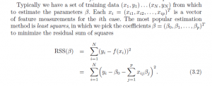
Following Hastie, Tibshirani, and Friedman, the Regression Sum of Squares (RSS) can be expressed,
The solution to this least squares error minimization problem can be stated in a matrix formula,
β= (XTX)-1XTY
where X is the data matrix, Here XT denotes the transpose of the matrix X.
Now ridge regression involves creating a penalty in the minimization of the squared errors designed to force down the absolute size of the regression coefficients. Thus, the minimization problem is
This also can be solved analytically in a closed matrix formula, similar to that for OLS –
βridge= (XTX-λІ)-1XTY
Here λ is a penalty or conditioning factor, and I is the identity matrix. This conditioning factor λ, it should be noted, is usually determined by cross-validation – holding back some sample data and testing the impact of various values of λ on the goodness of fit of the overall relationship on this holdout or test data.
Ridge Regression in Excel
So what sort of results can be obtained with ridge regression in the context of many predictors?
Consider the following toy example.
By construction, the true relationship is
y = 2x1 + 5x2+0.25x1x2+0.5x12+1.5x22+0.5x1x22+0.4x12x2+0.2x13+0.3x23
so the top row with the numbers in bold lists the “true” coefficients of the relationship.
Also, note that, strictly speaking, this underlying equation is not linear, since some exponents of explanatory variables are greater than 1, and there are cross products.
Still, for purposes of estimation we treat the setup as though the data come from ten separate explanatory variables, each weighted by separate coefficients.
Now, assuming no constant term and mean-centered data. the data matrix X is 6 rows by 10 columns, since there are six observations or cases and ten explanatory variables. Thus, the transpose XT is a 10 by 6 matrix. Accordingly, the product XTX is a 10 by 10 matrix, resulting in a 10 by 10 inverse matrix after the conditioning factor and identity matrix is added in to XTX.
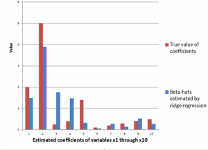
The ridge regression formula above, therefore, gives us estimates for ten beta-hats, as indicated in the following chart, using a λ or conditioning coefficient of .005.
The red bars indicate the true coefficient values, and the blue bars are the beta-hats estimated by the ridge regression formula.
As you can see, ridge regression does get into the zone in terms of these ten coefficients of this linear expression, but with only 6 observations, the estimate is very approximate.
The Kernel Trick
Note that in order to estimate the ten coefficients by ordinary ridge regression, we had to invert a 10 by 10 matrix XTX. We also can solve the estimation problem by inverting a 6 by 6 matrix, using the kernel trick, whose derivation is outlined in a paper by Exertate.
The key point is that kernel ridge regression is no different from ordinary ridge regression…except for an algebraic trick.
To show this, we applied the ridge regression formula to the 6 by 10 data matrix indicated above, estimating the ten coefficients, using a λ or conditioning coefficient of .005. These coefficients broadly resemble the true values.
The above matrix formula works for our linear expression in ten variables, which we can express as
y = β1x1+ β2x2+… + β10x10
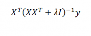
Now with suitable pre- and post-multiplications and resorting, it is possible to switch things around to arrive at another matrix formula,
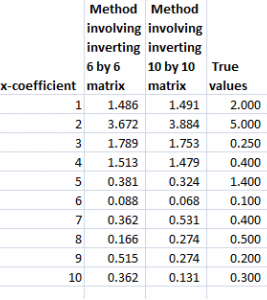
The following table shows beta-hats estimated by these two formulas are similar and compares them with the “true” values of the coefficients.
Differences in the estimates by these formulas relate strictly to issues at the level of numerical analysis and computation.
See also Exterkate et al “Nonlinear..” white paper.
Kernels
Notice that the ten variables could correspond to a Taylor expansion which might be used to estimate the value of a nonlinear function. This is important and illustrates the concept of a “kernel”.
Thus, designating K = XXT we find that the elements of K can be obtained without going through the indicated multiplication of these two matrices. This is because K is a polynomial kernel.
The second matrix formula listed just above involves inverting a smaller matrix, than the original formula – in our example, a 6 by 6, rather than a 10 by 10 matrix. This does not seem like a big deal with this toy example, but in Big Data and data mining applications, involving matrices with hundreds or thousands of rows and columns, the reduction in computation burden can be significant.
Summing Up
There is a great deal more that can be said about this example and the technique in general. Two big areas are (a) arriving at the estimate of the conditioning factor λ and (b) discussing the range of possible kernels that can be used, what makes a kernel a kernel, how to generate kernels from existing kernels, where Hilbert spaces come into the picture, and so forth.
But perhaps the important thing to remember is that ridge regression is one way to pry open the problem of many predictors, making it possible to draw on innumerable explanatory variables regardless of the size of the sample (within reason of course). Other techniques that do this include principal components regression and the lasso.
