Recently, Nate Silver boosted Bayesian methods in his popular book The Signal and the Noise – Why So Many Predictions Fail – But Some Don’t. I’m guessing the core application for Silver is estimating batting averages. Silver first became famous with PECOTA, a system for forecasting the performance of Major League baseball players.
Let’s assume a player’s probability p of getting a hit is constant over a season, but that it varies from year to year. He has up years, and down years. And let’s compare frequentist (gnarly word) and Bayesian approaches at the beginning of the season.
The frequentist approach is based on maximum likelihood estimation with the binomial formula
Here the n and the k in parentheses at the beginning of the expression stand for the combination of n things taken k at a time. That is, the number of possible ways of interposing k successes (hits) in n trials (times at bat) is the combination of n things taken k at a time (formula here).
If p is the player’s probability of hitting at bat, then the entire expression is the probability the player will have k hits in n times at bat.
The Frequentist Approach
There are a couple of ways to explain the frequentist perspective.
One is that this binomial expression is approximated to a higher and higher degree of accuracy by a normal distribution. This means that – with large enough n – the ratio of hits to total times at bat is the best estimate of the probability of a player hitting at bat – or k/n.
This solution to the problem also can be shown to follow from maximizing the likelihood of the above expression for any n and k. The large sample or asymptotic and maximum likelihood solutions are numerically identical.
The problem comes with applying this estimate early on in the season. So if the player has a couple of rough times at bat initially, the frequentist estimate of his batting average for the season at that point is zero.
The Bayesian Approach
The Bayesian approach is based on the posterior probability distribution for the player’s batting average. From Bayes Theorem, this is a product of the likelihood and a prior for the batting average.
Now generally, especially if we are baseball mavens, we have an idea of player X’s batting average. Say we believe it will be .34 – he’s going to have a great season, and did last year.
In this case, we can build that belief or information into a prior that is a beta distribution with two parameters α and β that generate a mean of α/(α+β).
In combination with the binomial likelihood function, this beta distribution prior combines algebraically into a closed form expression for another beta function with parameters which are adjusted by the values of k and n-k (the number of strike-outs). Note that walks (also being hit by the ball) do not count as times at bat.
This beta function posterior distribution then can be moved back to the other side of the Bayes equation when there is new information – another hit or strikeout.
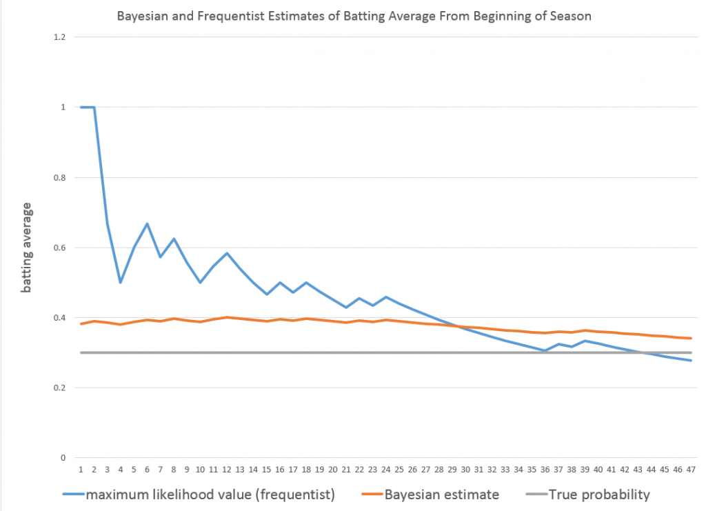
Taking the average of the beta posterior as the best estimate of p, then, we get successive approximations, such as shown in the following graph.
So the player starts out really banging ‘em, and the frequentist estimate of his batting average for that season starts at 100 percent. The Bayesian estimate on the other hand is conditioned by a belief that his batting average should be somewhere around 0.34. In fact, as the grey line indicates, his actual probability p for that year is 0.3. Both the frequentist and Bayesian estimates converge towards this value with enough times at bat.
I used α=33 and β=55 for the initial values of the Beta distribution.
See this for a great discussion of the intuition behind the Beta distribution.
This, then, is a worked example showing how Bayesian methods can include prior information, and have small sample properties which can outperform a frequentist approach.
Of course, in setting up this example in a spreadsheet, it is possible to go on and generate a large number of examples to explore just how often the Bayesian estimate beats the frequentist estimate in the early part of a Bernoulli process.
Which goes to show that what you might call the classical statistical approach – emphasizing large sample properties, covering all cases, still has legs.


