Category Archives: Monte Carlo simulation

Bayesian Methods in Biomedical Research

I’ve come across an interesting document – Guidance for the Use of Bayesian Statistics in Medical Device Clinical Trials developed by the Federal Drug Administration (FDA).

It’s billed as “Guidance for Industry and FDA Staff,” and provides recent (2010) evidence of the growing acceptance and success of Bayesian methods in biomedical research.

This document, which I’m just going to refer to as “the Guidance,” focuses on using Bayesian methods to incorporate evidence from prior research in clinical trials of medical equipment.

Bayesian statistics is an approach for learning from evidence as it accumulates. In clinical trials, traditional (frequentist) statistical methods may use information from previous studies only at the design stage. Then, at the data analysis stage, the information from these studies is considered as a complement to, but not part of, the formal analysis. In contrast, the Bayesian approach uses Bayes’ Theorem to formally combine prior information with current information on a quantity of interest. The Bayesian idea is to consider the prior information and the trial results as part of a continual data stream, in which inferences are being updated each time new data become available.

This Guidance focuses on medical devices and equipment, I think, because changes in technology can be incremental, and sometimes do not invalidate previous clinical trials of similar or earlier model equipment.

Thus,

When good prior information on clinical use of a device exists, the Bayesian approach may enable this information to be incorporated into the statistical analysis of a trial. In some circumstances, the prior information for a device may be a justification for a smaller-sized or shorter-duration pivotal trial.

Good prior information is often available for medical devices because of their mechanism of action and evolutionary development. The mechanism of action of medical devices is typically physical. As a result, device effects are typically local, not systemic. Local effects can sometimes be predictable from prior information on the previous generations of a device when modifications to the device are minor. Good prior information can also be available from studies of the device overseas. In a randomized controlled trial, prior information on the control can be available from historical control data.

The Guidance says that Bayesian methods are more commonly applied now because of computational advances – namely Markov Chain Monte Carlo (MCMC) sampling.

The Guidance also recommends that meetings be scheduled with the FDA for any Bayesian experimental design, where the nature of the prior information can be discussed.

An example clinical study is referenced in the Guidance – relating to a multi-frequency impedence breast scanner. This study combined clinical trials conducted in Israel with US trials,

Israelistudy

The Guidance provides extensive links to the literature and to WinBUGS where BUGS stands for Bayesian Inference Using Gibbs Sampling.

Bayesian Hierarchical Modeling

One of the more interesting sections in the Guidance is the discussion of Bayesian hierarchical modeling. Bayesian hierarchical modeling is a methodology for combining results from multiple studies to estimate safety and effectiveness of study findings. This is definitely an analysis-dependent approach, involving adjusting results of various studies, based on similarities and differences in covariates of the study samples. In other words, if the ages of participants were quite different in one study than in another, the results of the study might be adjusted for this difference (by regression?).

An example of Bayesian hierarchical modeling is provided in approval of a device called for Cervical Interbody Fusion Instrumentation.

The BAK/Cervical (hereinafter called the BAK/C) Interbody Fusion System is indicated for use in skeletally mature patients with degenerative disc disease (DDD) of the cervical spine with accompanying radicular symptoms at one disc level.

The Summary of the FDA approval for this device documents extensive Bayesian hierarchical modeling.

Bottom LIne

Stephen Goodman from the Stanford University Medical School writes in a recent editorial,

“First they ignore you, then they laugh at you, then they fight you, then you win,” a saying reportedly misattributed to Mahatma Ghandi, might apply to the use of Bayesian statistics in medical research. The idea that Bayesian approaches might be used to “affirm” findings derived from conventional methods, and thereby be regarded as more authoritative, is a dramatic turnabout from an era not very long ago when those embracing Bayesian ideas were considered barbarians at the gate. I remember my own initiation into the Bayesian fold, reading with a mixture of astonishment and subversive pleasure one of George Diamond’s early pieces taking aim at conventional interpretations of large cardiovascular trials of the early 80’s..It is gratifying to see that the Bayesian approach, which saw negligible application in biomedical research in the 80’s and began to get traction in the 90’s, is now not just a respectable alternative to standard methods, but sometimes might be regarded as preferable.

There’s a tremendous video provided by Medscape (not easily inserted directly here) involving an interview with one of the original and influential medical Bayesians – Dr. George Diamond of UCLA.

Diamond

URL: http://www.medscape.com/viewarticle/813984



Bayesian Methods in Forecasting and Data Analysis

The basic idea of Bayesian methods is outstanding. Here is a way of incorporating prior information into analysis, helping to manage, for example, small samples that are endemic in business forecasting.

What I am looking for, in the coming posts on this topic, is what difference does it make.

Bayes Theorem

Just to set the stage, consider the simple statement and derivation of Bayes Theorem –

BayesThm

Here A and B are events or occurrences, and P(.) is the probability (of the argument . ) function. So P(A) is the probability of event A. And P(A|B) is the conditional probability of event A, given that event B has occurred.

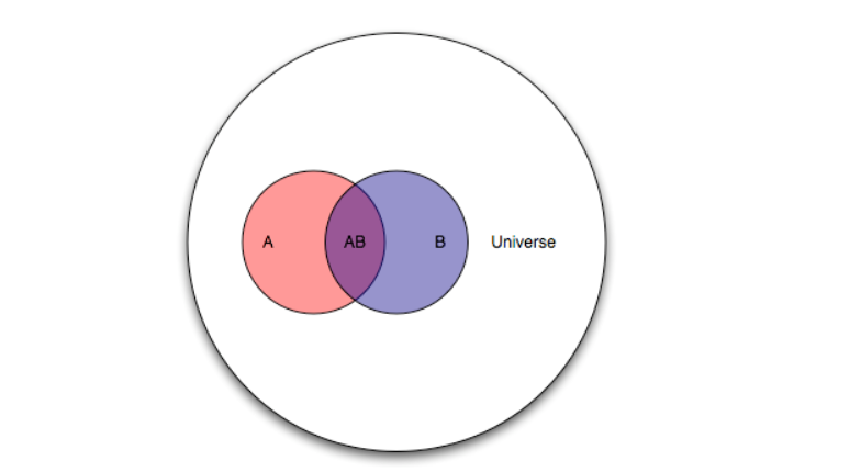
A Venn diagram helps.

Venn

Here, there is the universal set U, and the two subsets A and B. The diagram maps some type of event or belief space. So the probability of A or P(A) is the ratio of the areas A and U.

Then, the conditional probability of the occurrence of A, given the occurrence of B is the ratio of the area labeled AB to the area labeled B in the diagram. Also area AB is the intersection of the areas A and B or A ∩ B in set theory notation. So we have P(A|B)=P(A ∩ B)/P(B).

By the same logic, we can create the expression for P(B|A) = P(B ∩ A)/P(A).

Now to be mathematically complete here, we note that intersection in set theory is commutative, so A ∩ B = B ∩ A, and thus P(A ∩ B)=P(B|A)•P(A). This leads to the initially posed formulation of Bayes Theorem by substitution.

So Bayes Theorem, in its simplest terms, follows from the concept or definition of conditional probability – nothing more.

Prior and Posterior Distributions and the Likelihood Function

With just this simple formulation, one can address questions that are essentially what I call “urn problems.” That is, having drawn some number of balls of different colors from one of several sources (urns), what is the probability that the combination of, say, red and white balls drawn comes from, say, Urn 2? Some versions of even this simple setup seem to provide counter-intuitive values for the resulting P(A|B).

But I am interested primarily in forecasting and data analysis, so let me jump ahead to address a key interpretation of the Bayes Theorem.

Thus, what is all this business about prior and posterior distributions, and also the likelihood function?

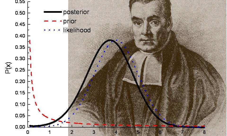
Well, considering Bayes Theorem as a statement of beliefs or subjective probabilities, P(A) is the prior distribution, and P(A|B) is the posterior distribution, or the probability distribution that follows revelation of the facts surrounding event (or group of events) B.

P(B|A) then is the likelihood function.

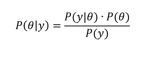
Now all this is more understandable, perhaps, if we reframe Bayes rule in terms of data y and parameters θ of some statistical model.

So we have

Bayes2

In this case, we have some data observations {y1, y2,…,yn}, and can have covariates x={x1,..,xk}, which could be inserted in the conditional probability of the data, given the parameters on the right hand side of the equation, as P(y|θ,x).

In any case, clear distinctions between the Bayesian and frequentist approach can be drawn with respect to the likelihood function P(y|θ).

So the frequentist approach focuses on maximizing the likelihood function with respect to the unknown parameters θ, which of course can be a vector of several parameters.

As one very clear overview says,

One maximizes the likelihood function L(·) with respect the parameters to obtain the maximum likelihood estimates; i.e., the parameter values most likely to have produced the observed data. To perform inference about the parameters, the frequentist recognizes that the estimated parameters ˆ result from a single sample, and uses the sampling distribution to compute standard errors, perform hypothesis tests, construct confidence intervals, and the like..

In the Bayesian perspective, the unknown parameters θ are treated as random variables, while the observations y are treated as fixed in some sense.

The focus of attention is then on how the observed data y changes the prior distribution P(θ) into the posterior distribution P(y|θ).

The posterior distribution, in essence, translates the likelihood function into a proper probability distribution over the unknown parameters, which can be summarized just as any probability distribution; by computing expected values, standard deviations, quantiles, and the like. What makes this possible is the formal inclusion of prior information in the analysis.

One difference then is that the frequentist approach optimizes the likelihood function with respect to the unknown parameters, while the Bayesian approach is more concerned with integrating the posterior distribution to obtain values for key metrics and parameters of the situation, after data vector y is taken into account.

Extracting Parameters From the Posterior Distribution

The posterior distribution, in other words, summarizes the statistical model of a phenomenon which we are analyzing, given all the available information.

That sounds pretty good, but the issue is that the result of all these multiplications and divisions on the right hand side of the equation can lead to a posterior distribution which is difficult to evaluate. It’s a probability distribution, for example, and thus some type of integral equation, but there may be no closed form solution.

Prior to Big Data and the muscle of modern computer computations, Bayesian statisticians spent a lot of time and energy searching out conjugate prior’s. Wikipedia has a whole list of these.

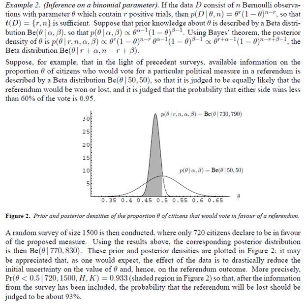
So the Beta distribution is a conjugate prior for a Bernoulli distribution – the familiar probability p of success and probability q of failure model (like coin-flipping, when p=q=0.5). This means simply that multiplying a Bernoulli likelihood function by an appropriate Beta distribution leads to a posterior distribution that is again a Beta distribution, and which can be integrated and, also, which supports a sort of loop of estimation with existing and then further data.

Here’s an example and prepare yourself for the flurry of symbolism –

BayesexampleB

Note the update of the distribution of whether the referendum is won or lost results in a much sharper distribution and increase in the probability of loss of the referendum.

Monte Carlo Methods

Stanislaus Ulam, along with John von Neumann, developed Monte Carlo simulation methods to address what might happen if radioactive materials were brought together in sufficient quantities and with sufficient emissions of neutrons to achieve a critical mass. That is, researchers at Los Alamos at the time were not willing to simply experiment to achieve this effect, and watch the unfolding.

Monte Carlo computation methods, thus, take complicated mathematical relationships and calculate final states or results from random assignments of values of the explanatory variables.

Two algorithms—the Gibbs sampling and Metropolis-Hastings algorithms— are widely used for applied Bayesian work, and both are Markov chain Monte Carlo methods.

The Markov chain aspect of the sampling involves selection of the simulated values along a path determined by prior values that have been sampled.

The object is to converge on the key areas of the posterior distribution.

The Bottom Line

It has taken me several years to comfortably grasp what is going on here with Bayesian statistics.

The question, again, is what difference does it make in forecasting and data analysis? And, also, if it made a difference in comparison with a frequentist interpretation or approach, would that be an entirely good thing?

A lot of it has to do with a reorientation of perspective. So some of the enthusiasm and combative qualities of Bayesians seems to come from their belief that their system of concepts is simply the only coherent one.

But there are a lot of medical applications, including some relating to trials of new drugs and procedures. What goes there? Is the representation that it is not necessary to take all this time required by the FDA to test a drug or procedure, when we can access prior knowledge and bring it to the table in evaluating outcomes?

Or what about forecasting applications? Is there something more productive about some Bayesian approaches to forecasting – something that can be measured in, for example, holdout samples or the like? Or I don’t know whether that violates the spirit of the approach – holdout samples.

I’m planning some posts on this topic. Let me know what you think.

Top picture from Los Alamos laboratories

Predicting the S&P 500 or the SPY Exchange-Traded Fund

By some lights, predicting the stock market is the ultimate challenge. Tremendous resources are dedicated to it – pundits on TV, specialized trading programs, PhD’s doing high-end quantitative analysis in hedge funds. And then, of course, theories of “rational expectations” and “efficient markets” deny the possibility of any consistent success at stock market prediction, on grounds that stock prices are basically random walks.

I personally have not dabbled much in forecasting the market, until about two months ago, when I grabbed a bunch of data on the S&P 500 and tried some regressions with lags on S&P 500 daily returns and daily returns from the VIX volatility index.

What I discovered is completely replicable, and also, so far as I can see, is not widely known.

An autoregressive time series model of S&P 500 or SPY daily returns, built with data from 1993 to early 2008, can outperform a Buy & Hold strategy initiated with out-of-sample data beginning January 2008 and carrying through to recent days.

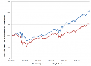
Here is a comparison of cumulative gains from a Buy & Hold strategy initiated January 23, 2008 with a Trading Strategy informed by my autoregressive (AR) model.

TradingStrategy1

So, reading this chart, investing $1000 January 23, 2008 and not touching this investment leads to cumulative returns of $1586.84 – that’s the Buy & Hold strategy.

The AR trading model, however, generates cumulative returns over this period of $2097.

The trading program based on the autoregressive model I am presenting here works like this. The AR model predicts the next day return for the SPY, based on the model coefficients (which I detail below) and the daily returns through the current day. So, if there is an element of unrealism, it is because the model is based on the daily returns computed on closing values day-by-day. But, obviously, you have to trade before the closing bell (in standard trading), so you need to use a estimate of the current day’s closing value obtained very close to the bell, before deciding whether to invest, sell, or buy SPY for the next day’s action.

But basically, assuming we can do this, perhaps seconds before the bell, and come close to an estimate of the current day closing price – the AR trading program is to buy SPY if the next day’s return is predicted to be positive – or if you currently hold SPY, to continue holding it. If the next day’s return is predicted to be negative, you sell your holdings.

It’s as simple as that.

So the AR model predicts daily returns on a one-day-ahead basis, using information on daily returns through the current trading day, plus the model coefficients.

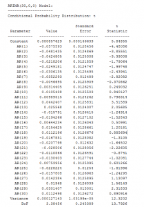
Speaking of which, here are the coefficients from the Matlab “printout.”

MatlabTM1

There are a couple of nuances here. First, these parameter values do not derive from an ordinary least squares (OLS) regression. Instead, they are produced by maximum likelihood estimation, assuming the underlying distribution is a t-distribution (not a Gaussian distribution).

The use of a t-distribution, the idea of which I got to some extent from Nassim Taleb’s new text-in-progress mentioned two posts ago, is motivated by the unusual distribution of residuals of an OLS regression of lagged daily returns.

The proof is in the pudding here, too, since the above coefficients work better than ones developed on the (manifestly incorrect) assumption that the underlying error distribution is Gaussian.

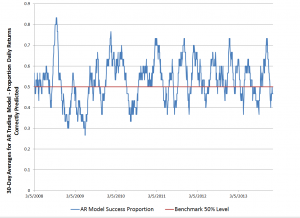
Here is a graph of the 30-day moving averages of the proportion of signs of daily returns correctly predicted by this model.

TPproportions

Overall, about 53 percent of the signs of the daily returns in this out-of-sample period are predicted correctly.

If you look at this graph, too, it’s clear there are some differences in performance over this period. Thus, the accuracy of the model took a dive in 2009, in the depths of the Great Recession. And, model performance achieved significantly higher success proportions in 2012 and early 2013, perhaps related to markets getting used to money being poured in by the Fed’s policies of quantitative easing.

Why This AR Model is Such a Big Deal

I find it surprising that a set of fixed coefficients applied to the past 30 values of the SPY daily returns continue to predict effectively, months and years after the end of the in-sample values.

And, I might add, it’s not clear that updating the AR model always improves the outcomes, although I can do more work on this and also on the optimal sample period generally.

Can this be a matter of pure chance? This has to be considered, but I don’t think so. Monte Carlo simulations of randomized trading indicate that there is a 95 percent chance or better than returns of $2097 in this period are not due to chance. In other words, if I decide to trade on a day based on a flip of a fair coin, heads I buy, tails I sell at the end of the day, it’s highly unlikely I will generate cumulative returns of $2097, given the SPY returns over this period.

The performance of this trading model holds up fairly well through December of last year, but degrades some in the first days of 2014.

I think this is a feather in the cap of forecasting, so to speak. Also, it seems to me that economists promoting ideas of market efficiency and rational expectations need to take these findings into account. Everything is extant. I have provided the coefficients. You can get the SPY daily return values from Yahoo Finance. You can calculate everything yourself to check. I’ve done this several times, slightly differently each time. This time I used Matlab, and its arima estimation procedures work well.

I’m not quite sure what to make of all this, but I think it’s important. Naturally, I am extending these results in my personal model-building, and I can report that extensions are possible. At the same time, no extension of this model I have seen achieves more than nearly 60 percent accuracy in predicting the direction of change or sign of the daily returns, so you are going to lose money sometimes applying these models. Day-trading is a risky business.