Category Archives: Uncategorized

Estimation and Variable Selection with Ridge Regression and the LASSO

I’ve posted on ridge regression and the LASSO (Least Absolute Shrinkage and Selection Operator) some weeks back.

Here I want to compare them in connection with variable selection  where there are more predictors than observations (“many predictors”).

1. Ridge regression does not really select variables in the many predictors situation. Rather, ridge regression “shrinks” all predictor coefficient estimates toward zero, based on the size of the tuning parameter λ. When ordinary least squares (OLS) estimates have high variability, ridge regression estimates of the betas may, in fact, produce lower mean square error (MSE) in prediction.

2. The LASSO, on the other hand, handles estimation in the many predictors framework and performs variable selection. Thus, the LASSO can produce sparse, simpler, more interpretable models than ridge regression, although neither dominates in terms of predictive performance. Both ridge regression and the LASSO can outperform OLS regression in some predictive situations – exploiting the tradeoff between variance and bias in the mean square error.

3. Ridge regression and the LASSO both involve penalizing OLS estimates of the betas. How they impose these penalties explains why the LASSO can “zero” out coefficient estimates, while ridge regression just keeps making them smaller. From
An Introduction to Statistical Learning

ridgeregressionOF

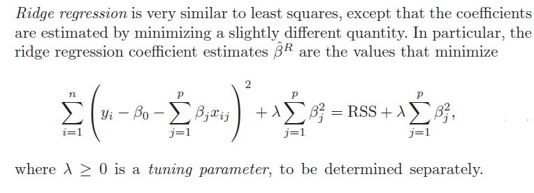
Similarly, the objective function for the LASSO procedure is outlined by An Introduction to Statistical Learning, as follows

LASSOobkf

4. Both ridge regression and the LASSO, by imposing a penalty on the regression sum of squares (RWW) shrink the size of the estimated betas. The LASSO, however, can zero out some betas, since it tends to shrink the betas by fixed amounts, as λ increases (up to the zero lower bound). Ridge regression, on the other hand, tends to shrink everything proportionally.

5.The tuning parameter λ in ridge regression and the LASSO usually is determined by cross-validation. Here are a couple of useful slides from Ryan Tibshirani’s Spring 2013 Data Mining course at Carnegie Mellon.

RTCV1

RTCV2

6.There are R programs which estimate ridge regression and lasso models and perform cross validation, recommended by these statisticians from Stanford and Carnegie Mellon. In particular, see glmnet at CRAN. Mathworks MatLab also has routines to do ridge regression and estimate elastic net models.

Here, for example, is R code to estimate the LASSO.

lasso.mod=glmnet(x[train,],y[train],alpha=1,lambda=grid)
plot(lasso.mod)
set.seed(1)
cv.out=cv.glmnet(x[train,],y[train],alpha=1)
plot(cv.out)
bestlam=cv.out$lambda.min
lasso.pred=predict(lasso.mod,s=bestlam,newx=x[test,])
mean((lasso.pred-y.test)^2)
out=glmnet(x,y,alpha=1,lambda=grid)
lasso.coef=predict(out,type=”coefficients”,s=bestlam)[1:20,]
lasso.coef
lasso.coef[lasso.coef!=0]

 What You Get

I’ve estimated quite a number of ridge regression and LASSO models, some with simulated data where you know the answers (see the earlier posts cited initially here) and other models with real data, especially medical or health data.

As a general rule of thumb, An Introduction to Statistical Learning notes,

 ..one might expect the lasso to perform better in a setting where a relatively small number of predictors have substantial coefficients, and the remaining predictors have coefficients that are very small or that equal zero. Ridge regression will perform better when the response is a function of many predictors, all with coefficients of roughly equal size.

The R program glmnet linked above is very flexible, and can accommodate logistic regression, as well as regression with continuous, real-valued dependent variables ranging from negative to positive infinity.


Changes to Businessforecastblog in 2014 – Where We Have Been, Where We Are Going

We’ve been struggling with a software glitch in WordPress, due to, we think, incompatibilities between plug-in’s and a new version of the blogging software. It’s been pretty intense. The site has been fully up, but there was no possibility of new posts, not even a notice to readers about what was happening. All this started just before Christmas and ended, basically, yesterday.

So greetings. Count on daily posts as rule, and I will get some of the archives accessible ASAP.

But, for now, a few words about my evolving perspective.

I came out of the trenches, so to speak, of sales, revenue, and new product forecasting, for enterprise information technology (IT) and, earlier, for public utilities and state and federal agencies. When I launched Businessforecastblog last year, my bias popped up in the secondary heading for the blog – with its reference to “data-limited contexts” – and in early posts on topics like “simple trending” and random walks.

longterm_study_of_market_trends

I essentially believed that most business and economic time series are basically one form or another of random walks, and that exponential smoothing is often the best forecasting approach in an applied context. Of course, this viewpoint can be bolstered by reference to research from the 1980’s by Nelson and Plosser and the M-Competitions. I also bought into a lazy consensus that it was necessary to have more observations than explanatory variables in order to estimate a multivariate regression. I viewed segmentation analysis, so popular in marketing research, as a sort of diversion from the real task of predicting responses of customers directly, based on their demographics, firmagraphics, and other factors.

So the press of writing frequent posts on business forecasting and related topics has led me to a learn a lot.

The next post to this blog, for example, will be about how “bagging” – from Bootstrap Aggregation – can radically reduce forecasting errors when there are only a few historical or other observations, but a large number of potential predictors. In a way, this provides a new solution to the problem of forecasting in data limited contexts.

This post also includes specific computations, in this case done in a spreadsheet. I’m big on actually computing stuff, where possible. I believe Elliot Shulman’s dictum, “you don’t really know something until you compute it.” And now I see how to include access to spreadsheets for readers, so there will be more of that.

Forecasting turning points is the great unsolved problem of business forecasting. That’s why I’m intensely interested in analysis of what many agree are asset bubbles. Bursting of the dot.com bubble initiated the US recession of 2001. Collapse of the housing market and exotic financial instrument bubbles in 2007 bought on the worst recession since World War II, now called the Great Recession. If it were possible to forecast the peak of various asset bubbles, like researchers such as Didier Sornette suggest, this would mean we would have some advance – perhaps only weeks of course – on the onset of the next major business turndown.

Along the way, there are all sorts of interesting sidelights relating to business forecasting and more generally predictive analytics. In fact, it’s clear that in the era of Big Data, data analytics can contribute to improvement of business processes – things like target marketing for customers – as well as perform less glitzy tasks of projecting sales for budget formulation and the like.

Email me at [email protected] if you want to receive PDF compilations on topics from the archives. I’m putting together compilations on New Methods and Asset Bubbles, for starters, in a week or so.