Ok, I am documenting and extending a method of forecasting stock market prices based on what I call Pvar models. Here Pvar stands for “proximity variable” – or, more specifically, variables based on the spread or difference between the opening price of a stock, ETF, or index, and the high or low of the previous period. These periods can be days, groups of days, weeks, months, and so forth.
I share features of these models and some representative output on this blog.
And, of course, I continue to have wider interests in forecasting controversies, issues, methods, as well as the global economy.
But for now, I’ve got hold of something, and since I appreciate your visits and comments, let’s talk about “scalability.”
Forecast Error and Data Frequency
Years ago, when I first heard of the M-competition (probably later than for some), I was intrigued by reports of how forecast error blows up “three or four periods in the forecast horizon,” almost no matter what the data frequency. So, if you develop a forecast model with monthly data, forecast error starts to explode three or four months into the forecast horizon. If you use quarterly data, you can push the error boundary out three or four quarters, and so forth.
I have not seen mention of this result so much recently, so my memory may be playing tricks.
But the basic concept seems sound. There is irreducible noise in data and in modeling. So whatever data frequency you are analyzing, it makes sense that forecast errors will start to balloon more or less at the same point in the forecast horizon – in terms of intervals of the data frequency you are analyzing.
Well, this concept seems emergent in forecasts of stock market prices, when I apply the analysis based on these proximity variables.
Prediction of Highs and Lows of Microsoft (MSFT) Stock at Different Data Frequencies
What I have discovered is that in order to predict over longer forecast horizons, when it comes to stock prices, it is necessary to look back over longer historical periods.
Here are some examples of scalability in forecasts of the high and low of MSFT.
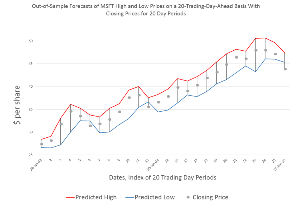
Forecasting 20 trading days ahead, you get this type of chart for recent 20-day-periods.
One of the important things to note is that these are out-of-sample forecasts, and that, generally, they encapsulate the actual closing prices for these 20 trading day periods.
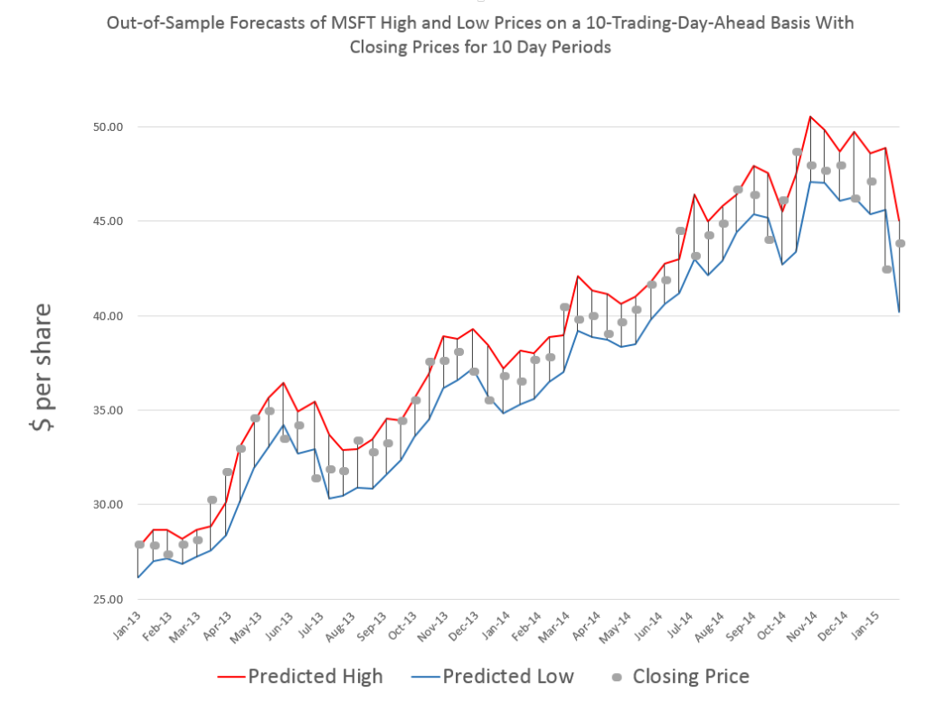
Here is a comparable chart for 10 trading days.
Same data, forecasts also are out-of-sample, and, of course, there are more closing prices to chart, too.
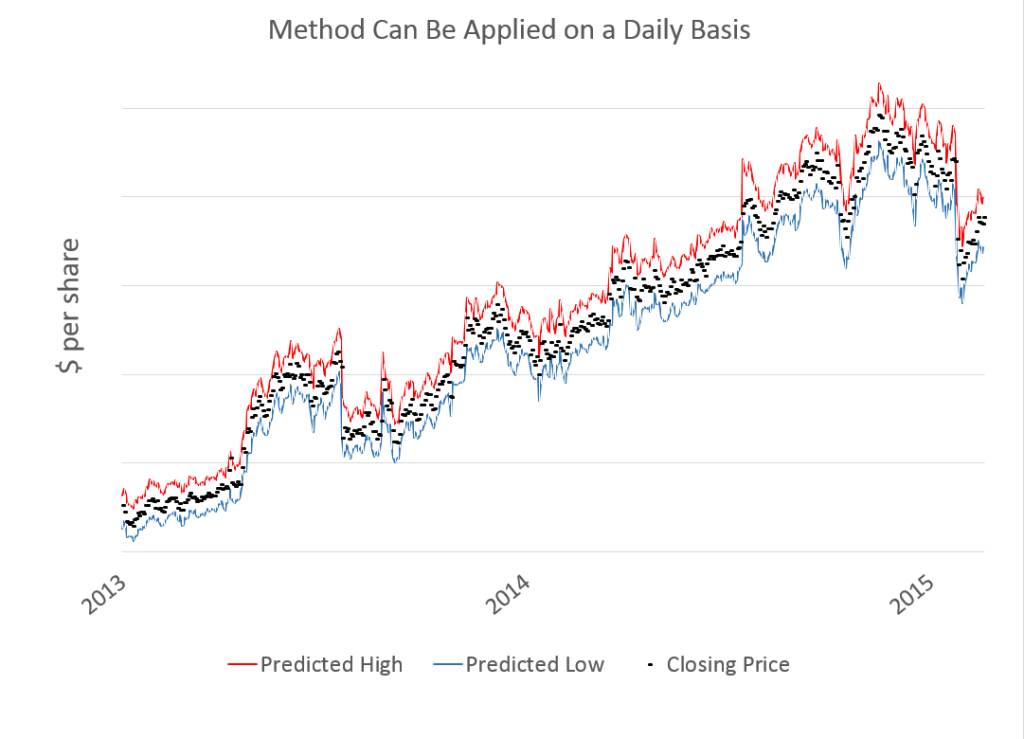
Finally, here is a very busy chart with forecasts by trading day.
Now there are several key points to take away from these charts.
First, the predictions of MSFT high and low prices for these periods are developed by similar forecast models, at least with regard to the specification of explanatory variables. Also, the Pvar method works for specific stocks, as well as for stock market indexes and ETF’s that might track them.
However, and this is another key point, the definitions of these variables shift with the periods being considered.
So the high for MSFT by trading day is certainly different from the MSFT high over groups of 20 trading days, and so forth.
In any case, there is remarkable scalability with Pvar models, all of which suggests they capture some of the interplay between long and shorter term trading.
While I am handing out conjectures, here is another one.
I think it will be possible to conduct a “causal analysis” to show that the Pvar variables reflect or capture trader actions, and that these actions tend to drive the market.


In my own experience with data at different frequencies (energy prices or renewable production), I found that there is short as well as long-range information in many time series. If you somehow manage to filter out the long range signal in high frequency data, you can blend the short with the long term forecasts and improve forecasting accuracy altogether.