Evaluating and predicting seasonal variation is a core competence of forecasting, dating back to the 1920’s or earlier. It’s essential to effective business decisions. For example, as the fiscal year unfolds, the question is “how are we doing?” Will budget forecasts come in on target, or will more (or fewer) resources be required? Should added resources be allocated to Division X and taken away from Division Y? To answer such questions, you need a within-year forecast model, which in most organizations involves quarterly or monthly seasonal components or factors.

Seasonal adjustment, on the other hand, is more mysterious. The purpose is more interpretive. Thus, when the Bureau of Labor Statistics (BLS) or Bureau of Economic Analysis (BEA) announce employment or other macroeconomic numbers, they usually try to take out special effects (the “Christmas effect”) that purportedly might mislead readers of the Press Release. Thus, the series we hear about typically are “seasonally adjusted.”

You can probably sense my bias. I almost always prefer data that is not seasonally adjusted in developing forecasting models. I just don’t know what magic some agency statistician has performed on a series – whether artifacts have been introduced, and so forth.

On the other hand, I take the methods of identifying seasonal variation quite seriously. These range from Buys-Ballot tables and seasonal dummy variables to methods based on moving averages, trigonometric series (Fourier analysis), and maximum likelihood estimation.

Identifying seasonal variation can be fairly involved mathematically.

But there are some simple reality tests.

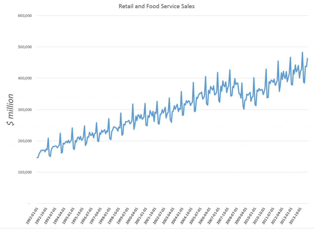
Take this US retail and food service sales series, for example.

Here you see the highly regular seasonal movement around a trend which, at times, is almost straight-line.

Are these additive or multiplicative seasonal effects? If we separate out the trend and the seasonal effects, do we add them or are the seasonal effects “factors” which multiply into the level for a month?

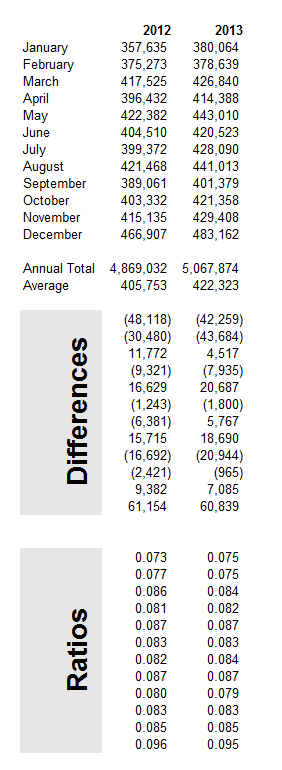
Well, for starters, we can re-arrange this time series into a kind of Buys-Ballot table. Here I only show the last two years.

The point is that we look at the differences between the monthly values in a year and the average for that year. Also, we calculate the ratios of each month to the annual total.

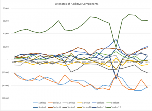
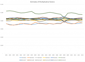
The issue is which of these numbers is most stable over the data period, which extends back to 1992 (click to enlarge).

Now here Series N relates to the Nth month, e.g. Series 12 = December.

It seems pretty clear that the multiplicative factors are more stable than the additive components in two senses. First, some additive components have a more pronounced trend; secondly, the variability of the additive components around this trend is greater.

This gives you a taste of some quick methods to evaluate aspects of seasonality.

Of course, there can be added complexities. What if you have daily data, or suppose there are other recurrent relationships. Then, trig series may be your best bet.

What if you only have two, three, or four years of data? Well, this interesting problem is frequently encountered in practical applications.

I’m trying to sort this material into posts for this coming week, along with stuff on controversies that swirl around the seasonal adjustment of macro time series, such as employment and real GDP.

Stay tuned.

Top image from http://www.livescience.com/25202-seasons.html