Category Archives: Granger causality

Semiconductor Cycles

I’ve been exploring cycles in the semiconductor, computer and IT industries generally for quite some time.

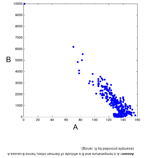
Here is an exhibit I prepared in 2000 for a magazine serving the printed circuit board industry.

semicycle

The data come from two sources – the Semiconductor Industry Association (SIA) World Semiconductor Trade Statistics database and the Census Bureau manufacturing series for computer equipment.

This sort of analytics spawned a spate of academic research, beginning more or less with the work of Tan and Mathews in Australia.

One of my favorites is a working paper released by DRUID – the Danish Research Unit for Industrial Dynamics called Cyclical Dynamics in Three Industries. Tan and Mathews consider cycles in semiconductors, computers, and what they call the flat panel display industry. They start with quoting “industry experts” and, specifically, some of my work with Economic Data Resources on the computer (PC) cycle. These researchers went on to publish in the Journal of Business Research and Technological Forecasting and Social Change in 2010. A year later in 2011, Tan published an interesting article on the sequencing of cyclical dynamics in semiconductors.

Essentially, the appearance of cycles and what I have called quasi-cycles or pseudo-cycles in the semiconductor industry and other IT categories, like computers, result from the interplay of innovation, investment, and pricing. In semiconductors, for example, Moore’s law – which everyone always predicts will fail at some imminent future point – indicates that continuing miniaturization will lead to periodic reductions in the cost of information processing. At some point in the 1980’s, this cadence was firmly established by introductions of new microprocessors by Intel roughly every 18 months. The enhanced speed and capacity of these microprocessors – the “central nervous system” of the computer – was complemented by continuing software upgrades, and, of course, by the movement to graphical interfaces with Windows and the succession of Windows releases.

Back along the supply chain, semiconductor fabs were retooling periodically to produce chips with more and more transitors per volume of silicon. These fabs were, simply put, fabulously expensive and the investment dynamics factors into pricing in semiconductors. There were famous gluts, for example, of memory chips in 1996, and overall the whole IT industry led the recession of 2001 with massive inventory overhang, resulting from double booking and the infamous Y2K scare.

Statistical Modeling of IT Cycles

A number of papers, summarized in Aubrey deploy VAR (vector autoregression) models to capture leading indicators of global semiconductor sales. A variant of these is the Bayesian VAR or BVAR model. Basically, VAR models sort of blindly specify all possible lags for all possible variables in a system of autoregressive models. Of course, some cutoff point has to be established, and the variables to be included in the VAR system have to be selected by one means or another. A BVAR simply reduces the number of possibilities by imposing, for example, sign constraints on the resulting coefficients, or, more ambitiously, employs some type of prior distribution for key variables.

Typical variables included in these models include:

  • WSTS monthly semiconductor shipments (now by subscription only from SIA)
  • Philadelphia semiconductor index (SOX) data
  • US data on various IT shipments, orders, inventories from M3
  • data from SEMI, the association of semiconductor equipment manufacturers

Another tactic is to filter out low and high frequency variability in a semiconductor sales series with something like the Hodrick-Prescott (HP) filter, and then conduct a spectral analysis.

Does the Semiconductor/Computer/IT Cycle Still Exist?

I wonder whether academic research into IT cycles is a case of “redoubling one’s efforts when you lose sight of the goal,” or more specifically, whether new configurations of forces are blurring the formerly fairly cleanly delineated pulses in sales growth for semiconductors, computers, and other IT hardware.

“Hardware” is probably a key here, since there have been big changes since the 1990’s and early years of this brave new century.

For one thing, complementarities between software and hardware upgrades seem to be breaking down. This began in earnest with the development of virtual servers – software which enabled many virtual machines on the same hardware frame, in part because the underlying circuitry was so massively powerful and high capacity now. Significant declines in the growth of sales of these machines followed on wide deployment of this software designed to achieve higher efficiencies of utilization of individual machines.

Another development is cloud computing. Running the data side of things is gradually being taken away from in-house IT departments in companies and moved over to cloud computing services. Of course, critical data for a company is always likely to be maintained in-house, but the need for expanding the number of big desktops with the number of employees is going away – or has indeed gone away.

At the same time, tablets, Apple products and Android machines, created a wave of destructive creation in people’s access to the Internet, and, more and more, for everyday functions like keeping calendars, taking notes, even writing and processing photos.

But note – I am not studding this discussion with numbers as of yet.

I suspect that underneath all this change it should be possible to identify some IT invariants, perhaps in usage categories, which continue to reflect a kind of pulse and cycle of activity.

Causal Discovery

So there’s a new kid on the block, really a former resident who moved back to the neighborhood with spiffy new toys – causal discovery.

Competitions and challenges give a flavor of this rapidly developing field – for example, the Causality Challenge #3: Cause-effect pairs, sponsored by a list of pre-eminent IT organizations and scientific societies (including Kaggle).

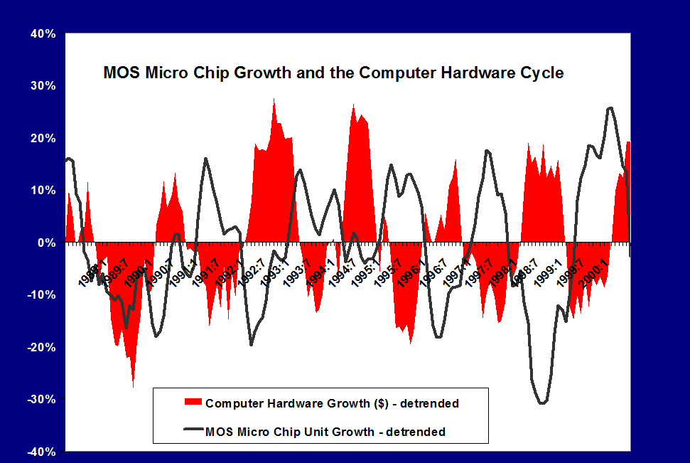
By way of illustration, B → A but A does not cause B – Why?

Kagglealttemp

These data, as the flipped answer indicates, are temperature and altitude of German cities. So altitude causes temperature, but temperature obviously does not cause altitude.

The non-linearity in the scatter diagram is a clue. Thus, values of variable A above about 130 map onto more than one value of B, which is problematic from conventional definition of causality. One cause should not have two completely different effects, unless there are confounding variables.

It’s a little fuzzy, but the associated challenge is very interesting, and data pairs still are available.

We provide hundreds of pairs of real variables with known causal relationships from domains as diverse as chemistry, climatology, ecology, economy, engineering, epidemiology, genomics, medicine, physics. and sociology. Those are intermixed with controls (pairs of independent variables and pairs of variables that are dependent but not causally related) and semi-artificial cause-effect pairs (real variables mixed in various ways to produce a given outcome).  This challenge is limited to pairs of variables deprived of their context.

Asymmetries As Clues to Causal Direction of Influence

The causal direction in the graph above is suggested by the non-invertibility of the functional relationship between B and A.

Another clue from reversing the direction of causal influence relates to the error distributions of the functional relationship between pairs of variables. This occurs when these error distributions are non-Gaussian, as Patrik Hoyer and others illustrate in Nonlinear causal discovery with additive noise models.

The authors present simulation and empirical examples.

Their first real-world example comes from data on eruptions of the Old Faithful geyser in Yellowstone National Park in the US.

OldFaithful Hoyer et al write,

The first dataset, the “Old Faithful” dataset [17] contains data about the duration of an eruption and the time interval between subsequent eruptions of the Old Faithful geyser in Yellowstone National Park, USA. Our method obtains a p-value of 0.5 for the (forward) model “current duration causes next interval length” and a p-value of 4.4 x 10⁻⁹ for the (backward) model “next interval length causes current duration”. Thus, we accept the model where the time interval between the current and the next eruption is a function of the duration of the current eruption, but reject the reverse model. This is in line with the chronological ordering of these events. Figure 3 illustrates the data, the forward and backward fit and the residuals for both fits. Note that for the forward model, the residuals seem to be independent of the duration, whereas for the backward model, the residuals are clearly dependent on the interval length.

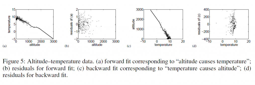
Then, they too consider temperature and altitude pairings.

tempaltHere, the correct model – altitude causes temperature – results in a much more random scatter of residuals, than the reverse direction model.

Patrik Hoyer and Aapo Hyvärinen are a couple of names from this Helsinki group of researchers whose papers are interesting to read and review.

One of the early champions of this resurgence of interest in causality works from a department of philosophy – Peter Spirtes. It’s almost as if the discussion of causal theory were relegated to philosophy, to be revitalized by machine learning and Big Data:

The rapid spread of interest in the last three decades in principled methods of search or estimation of causal relations has been driven in part by technological developments, especially the changing nature of modern data collection and storage techniques, and the increases in the processing power and storage capacities of computers. Statistics books from 30 years ago often presented examples with fewer than 10 variables, in domains where some background knowledge was plausible. In contrast, in new domains such as climate research (where satellite data now provide daily quantities of data unthinkable a few decades ago), fMRI brain imaging, and microarray measurements of gene expression, the number of variables can range into the tens of thousands, and there is often limited background knowledge to reduce the space of alternative causal hypotheses. Even when experimental interventions are possible, performing the many thousands of experiments that would be required to discover causal relationships between thousands or tens of thousands of variables is often not practical. In such domains, non-automated causal discovery techniques from sample data, or sample data together with a limited number of experiments, appears to be hopeless, while the availability of computers with increased processing power and storage capacity allow for the practical implementation of computationally intensive automated search algorithms over large search spaces.

Introduction to Causal Inference

Granger Causality

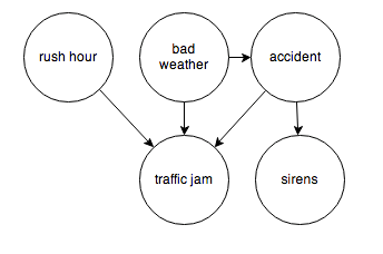
After review, I have come to the conclusion that from a predictive and operational standpoint, causal explanations translate to directed graphs, such as the following:

causegraph

And I think it is interesting the machine learning community focuses on causal explanations for “manipulation” to guide reactive and interactive machines, and that directed graphs (or perhaps a Bayesian networks) are a paramount concept.

Keep that thought, and consider “Granger causality.”

This time series concept is well explicated in C.W.J. Grangers’ 2003 Nobel Prize lecture – which motivates its discovery and links with cointegration.

An earlier concept that I was concerned with was that of causality. As a postdoctoral student in Princeton in 1959–1960, working with Professors John Tukey and Oskar Morgenstern, I was involved with studying something called the “cross-spectrum,” which I will not attempt to explain. Essentially one has a pair of inter-related time series and one would like to know if there are a pair of simple relations, first from the variable X explaining Y and then from the variable Y explaining X. I was having difficulty seeing how to approach this question when I met Dennis Gabor who later won the Nobel Prize in Physics in 1971. He told me to read a paper by the eminent mathematician Norbert Wiener which contained a definition that I might want to consider. It was essentially this definition, somewhat refined and rounded out, that I discussed, together with proposed tests in the mid 1960’s.

The statement about causality has just two components: 1. The cause occurs before the effect; and 2. The cause contains information about the effect that that is unique, and is in no other variable.

A consequence of these statements is that the causal variable can help forecast the effect variable after other data has first been used. Unfortunately, many users concentrated on this forecasting implication rather than on the original definition. At that time, I had little idea that so many people had very fixed ideas about causation, but they did agree that my definition was not “true causation” in their eyes, it was only “Granger causation.” I would ask for a definition of true causation, but no one would reply. However, my definition was pragmatic and any applied researcher with two or more time series could apply it, so I got plenty of citations. Of course, many ridiculous papers appeared.

When the idea of cointegration was developed, over a decade later, it became clear immediately that if a pair of series was cointegrated then at least one of them must cause the other. There seems to be no special reason why there two quite different concepts should be related; it is just the way that the mathematics turned out

In the two-variable case, suppose we have time series Y={y1,y2,…,yt} and X = {x1,..,xt}. Then, there are, at the outset, two cases, depending on whether Y and X are stationary or nonstationary. The classic case is where we have an autoregressive relationship for yt,

yt = a0+a1yt-1+..+akyt-k

and this relationship can be shown to be a weaker predictor than


yt = a0+a1yt-1+..+akyt-k + b0+b1xt-1+..+bmxt-m

In this case, we say that X exhibits Granger causality with respect to Y.

Of course, if Y and X are nonstationary time series, autoregressive predictive equations make no sense, and instead we have the case of cointegration of time series, where in the two-variable case,

yt=φxt-1+ut

and the series of residuals ut are reduced to a white noise process.

So these cases follow what good old Wikipedia says,

A time series X is said to Granger-cause Y if it can be shown, usually through a series of t-tests and F-tests on lagged values of X (and with lagged values of Y also included), that those X values provide statistically significant information about future values of Y.

There are a number of really interesting extensions of this linear case, discussed in a recent survey paper.

Stern points out that the main enemies or barriers to establishing causal relations are endogeneity and omitted variables.

So I find that margin loans and the level of the S&P 500 appear to be mutually interrelated. Thus, it is forecasts of the S&P 500 can be improved with lagged values of margin loans, and you can improve forecasts of the monthly total of margin loans with lagged values of the S&P 500 – at least over broad ranges of time and in the period since 2008. The predictions of the S&P 500 with lagged values of margin loans, however, are marginally more powerful or accurate predictions.

Stern gives a colorful example where an explanatory variable is clearly exogenous and appears to have a significant effect on the dependent variable and yet theory suggests that the relationship is spurious and due to omitted variables that happen to be correlated with the explanatory variable in question.

Westling (2011) regresses national economic growth rates on average reported penis lengths and other variables and finds that there is an inverted U shape relationship between economic growth and penis length from 1960 to 1985. The growth maximizing length was 13.5cm, whereas the global average was 14.5cm. Penis length would seem to be exogenous but the nature of this relationship would have changed over time as the fastest growing region has changed from Europe and its Western Offshoots to Asia. So, it seems that the result is likely due to omitted variables bias.

Here Stern notes that Westling’s data indicates penis length is lowest in Asia and greatest in Africa with Europe and its Western Offshoots having intermediate lengths.

There’s a paper which shows stock prices exhibit Granger causality with respect to economic growth in the US, but vice versa does not obtain. This is a good illustration of the careful ste-by-step in conducting this type of analysis, and how it is in fact fraught with issues of getting the number of lags exactly right and avoiding big specification problems.

Just at the moment when it looks as if the applications of Granger causality are petering out in economics, neuroscience rides to the rescue. I offer you a recent article from a journal in computation biology in this regard – Measuring Granger Causality between Cortical Regions from Voxelwise fMRI BOLD Signals with LASSO.

Here’s the Abstract:

Functional brain network studies using the Blood Oxygen-Level Dependent (BOLD) signal from functional Magnetic Resonance Imaging (fMRI) are becoming increasingly prevalent in research on the neural basis of human cognition. An important problem in functional brain network analysis is to understand directed functional interactions between brain regions during cognitive performance. This problem has important implications for understanding top-down influences from frontal and parietal control regions to visual occipital cortex in visuospatial attention, the goal motivating the present study. A common approach to measuring directed functional interactions between two brain regions is to first create nodal signals by averaging the BOLD signals of all the voxels in each region, and to then measure directed functional interactions between the nodal signals. Another approach, that avoids averaging, is to measure directed functional interactions between all pairwise combinations of voxels in the two regions. Here we employ an alternative approach that avoids the drawbacks of both averaging and pairwise voxel measures. In this approach, we first use the Least Absolute Shrinkage Selection Operator (LASSO) to pre-select voxels for analysis, then compute a Multivariate Vector AutoRegressive (MVAR) model from the time series of the selected voxels, and finally compute summary Granger Causality (GC) statistics from the model to represent directed interregional interactions. We demonstrate the effectiveness of this approach on both simulated and empirical fMRI data. We also show that averaging regional BOLD activity to create a nodal signal may lead to biased GC estimation of directed interregional interactions. The approach presented here makes it feasible to compute GC between brain regions without the need for averaging. Our results suggest that in the analysis of functional brain networks, careful consideration must be given to the way that network nodes and edges are defined because those definitions may have important implications for the validity of the analysis.

So Granger causality is still a vital concept, despite its probably diminishing use in econometrics per se.

Let me close with this thought and promise a future post on the Kaggle and machine learning competitions on identifying the direction of causality in pairs of variables without context.

Correlation does not imply causality—you’ve heard it a thousand times. But causality does imply correlation.