Category Archives: forecast competitions

Bagging Exponential Smoothing Forecasts

Bergmeir, Hyndman, and Benıtez (BHB) successfully combine two powerful techniques – exponential smoothing and bagging (bootstrap aggregation) – in ground-breaking research.

I predict the forecasting system described in Bagging Exponential Smoothing Methods using STL Decomposition and Box-Cox Transformation will see wide application in business and industry forecasting.

These researchers demonstrate their algorithms for combining exponential smoothing and bagging outperform all other forecasting approaches in the M3 forecasting competition database for monthly time series, and do better than many approaches for quarterly and annual data. Furthermore, the BHB approach can be implemented with extant routines in the programming language R.

This table compares bagged exponential smoothing with other approaches on monthly data from the M3 competition.

BaggedES

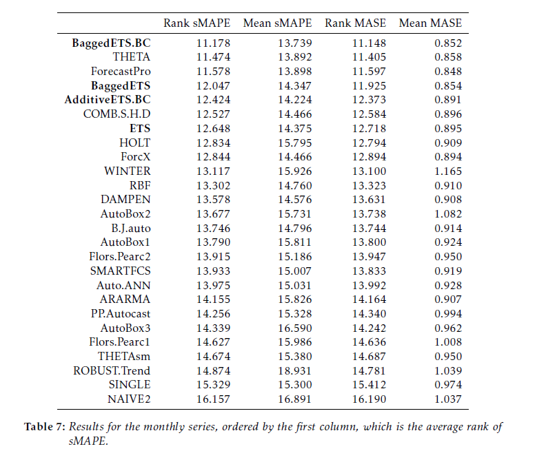
Here BaggedETS.BC refers to a variant of the bagged exponential smoothing model which uses a Box Cox transformation of the data to reduce the variance of model disturbances, The error metrics are the symmetric mean absolute percentage error (sMAPE) and the mean absolute scaled error (MASE). These are calculated for applications of the various models to out-of-sample, holdout, or test sample data from each of 1428 monthly time series in the competition.

See the online text by Hyndman and Athanasopoulos for motivations and discussions of these error metrics.

The BHB Algorithm

In a nutshell, here is the BHB description of their algorithm.

After applying a Box-Cox transformation to the data, the series is decomposed into trend, seasonal and remainder components. The remainder component is then bootstrapped using the MBB, the trend and seasonal components are added back, and the Box-Cox transformation is inverted. In this way, we generate a random pool of similar bootstrapped time series. For each one of these bootstrapped time series, we choose a model among several exponential smoothing models, using the bias-corrected AIC. Then, point forecasts are calculated using all the different models, and the resulting forecasts are averaged.

The MBB is the moving block bootstrap. It involves random selection of blocks of the remainders or residuals, preserving the time sequence and, hence, autocorrelation structure in these residuals.

Several R routines supporting these algorithms have previously been developed by Hyndman et al. In particular, the ets routine developed by Hyndman and Khandakar fits 30 different exponential smoothing models to a time series, identifying the optimal model by an Akaike information criterion.

Some Thoughts

This research lays out an almost industrial-scale effort to extract more information for prediction purposes from time series, and at the same time to use an applied forecasting workhorse – exponential smoothing.

Exponential smoothing emerged as a forecasting technique in applied contexts in the 1950’s and 1960’s. The initial motivation was error correction from forecasts of arbitrary origin, instead of an underlying stochastic model. Only later were relationships between exponential smoothing and time series processes, such as random walks, revealed with the work of Muth and others.

The M-competitions, initially organized in the 1970’s, gave exponential smoothing a big boost, since, by some accounts, exponential smoothing “won.” This is one of the sources of the meme – simpler models beat more complex models.

Then, at the end of the 1990’s, Makridakis and others organized a penultimate M-competition which was, in fact, won by the automatic forecasting software program Forecast Pro. This program typically compares ARIMA and exponential smoothing models, picking the best model through proprietary optimization of the parameters and tests on holdout samples. As in most sales and revenue forecasting applications, the underlying data are time series.

While all this was going on, the machine learning community was ginning up new and powerful tactics, such as bagging or bootstrap aggregation. Bagging can be a powerful technique for focusing on parameter estimates which are otherwise masked by noise.

So this application and research builds interestingly on a series of efforts by Hyndman and his associates and draws in a technique that has been largely confined to machine learning and data mining.

It is really almost the first of its kind – where bagging applications to time series forecasting have been less spectacularly successful than in cross-sectional regression modeling, for example.

A future post here will go through the step-by-step of this approach using some specific and familiar time series from the M competition data.

Causal Discovery

So there’s a new kid on the block, really a former resident who moved back to the neighborhood with spiffy new toys – causal discovery.

Competitions and challenges give a flavor of this rapidly developing field – for example, the Causality Challenge #3: Cause-effect pairs, sponsored by a list of pre-eminent IT organizations and scientific societies (including Kaggle).

By way of illustration, B → A but A does not cause B – Why?

Kagglealttemp

These data, as the flipped answer indicates, are temperature and altitude of German cities. So altitude causes temperature, but temperature obviously does not cause altitude.

The non-linearity in the scatter diagram is a clue. Thus, values of variable A above about 130 map onto more than one value of B, which is problematic from conventional definition of causality. One cause should not have two completely different effects, unless there are confounding variables.

It’s a little fuzzy, but the associated challenge is very interesting, and data pairs still are available.

We provide hundreds of pairs of real variables with known causal relationships from domains as diverse as chemistry, climatology, ecology, economy, engineering, epidemiology, genomics, medicine, physics. and sociology. Those are intermixed with controls (pairs of independent variables and pairs of variables that are dependent but not causally related) and semi-artificial cause-effect pairs (real variables mixed in various ways to produce a given outcome).  This challenge is limited to pairs of variables deprived of their context.

Asymmetries As Clues to Causal Direction of Influence

The causal direction in the graph above is suggested by the non-invertibility of the functional relationship between B and A.

Another clue from reversing the direction of causal influence relates to the error distributions of the functional relationship between pairs of variables. This occurs when these error distributions are non-Gaussian, as Patrik Hoyer and others illustrate in Nonlinear causal discovery with additive noise models.

The authors present simulation and empirical examples.

Their first real-world example comes from data on eruptions of the Old Faithful geyser in Yellowstone National Park in the US.

OldFaithful Hoyer et al write,

The first dataset, the “Old Faithful” dataset [17] contains data about the duration of an eruption and the time interval between subsequent eruptions of the Old Faithful geyser in Yellowstone National Park, USA. Our method obtains a p-value of 0.5 for the (forward) model “current duration causes next interval length” and a p-value of 4.4 x 10⁻⁹ for the (backward) model “next interval length causes current duration”. Thus, we accept the model where the time interval between the current and the next eruption is a function of the duration of the current eruption, but reject the reverse model. This is in line with the chronological ordering of these events. Figure 3 illustrates the data, the forward and backward fit and the residuals for both fits. Note that for the forward model, the residuals seem to be independent of the duration, whereas for the backward model, the residuals are clearly dependent on the interval length.

Then, they too consider temperature and altitude pairings.

tempaltHere, the correct model – altitude causes temperature – results in a much more random scatter of residuals, than the reverse direction model.

Patrik Hoyer and Aapo Hyvärinen are a couple of names from this Helsinki group of researchers whose papers are interesting to read and review.

One of the early champions of this resurgence of interest in causality works from a department of philosophy – Peter Spirtes. It’s almost as if the discussion of causal theory were relegated to philosophy, to be revitalized by machine learning and Big Data:

The rapid spread of interest in the last three decades in principled methods of search or estimation of causal relations has been driven in part by technological developments, especially the changing nature of modern data collection and storage techniques, and the increases in the processing power and storage capacities of computers. Statistics books from 30 years ago often presented examples with fewer than 10 variables, in domains where some background knowledge was plausible. In contrast, in new domains such as climate research (where satellite data now provide daily quantities of data unthinkable a few decades ago), fMRI brain imaging, and microarray measurements of gene expression, the number of variables can range into the tens of thousands, and there is often limited background knowledge to reduce the space of alternative causal hypotheses. Even when experimental interventions are possible, performing the many thousands of experiments that would be required to discover causal relationships between thousands or tens of thousands of variables is often not practical. In such domains, non-automated causal discovery techniques from sample data, or sample data together with a limited number of experiments, appears to be hopeless, while the availability of computers with increased processing power and storage capacity allow for the practical implementation of computationally intensive automated search algorithms over large search spaces.

Introduction to Causal Inference

Sayings of the Top Macro Forecasters

Yesterday, I posted the latest Bloomberg top twenty US macroeconomic forecaster rankings, also noting whether this current crop made it into the top twenty in previous “competitions” for November 2010-November 2012 or November 2009-November 2011.

It turns out the Bloomberg top twenty is relatively stable. Seven names or teams on the 2014 list appear in both previous competitions. Seventeen made it into the top twenty at least twice in the past three years.

But who are these people and how can we learn about their forecasts on a real-time basis?

Well, as you might guess, this is a pretty exclusive club. Many are Chief Economists and company Directors in investment advisory organizations serving private clients. Several did a stint on the staff of the Federal Reserve earlier in their career. Their public interface is chiefly through TV interviews, especially Bloomberg TV, or other media coverage.

I found a couple of exceptions, however – Michael Carey and Russell Price.

Michael Carey and Crédit Agricole

Michael Carey is Chief Economist North America Crédit Agricole CIB. He ranked 14, 7, and 5, based on his average scores for his forecasts of the key indicators in these three consecutive competitions. He apparently is especially good on employment forecasts.

MikeCarey

Carey is a lead author for a quarterly publication from Crédit Agricole called Prospects Macro.

The Summary for the current issue (1st Quarter 2014) caught my interest –

On the economic trend front, an imperfect normalisation seems to be getting underway. One may talk about a normalisation insofar as – unlike the two previous financial years – analysts have forecast a resumption of synchronous growth in the US, the Eurozone and China. US growth is forecast to rise from 1.8% in 2013 to 2.7%; Eurozone growth is slated to return to positive territory, improving from -0.4% to +1.0%; while Chinese growth is forecast to dip slightly, from 7.7% to 7.2%, which does not appear unwelcome nor requiring remedial measures. The imperfect character of the forecast normalisation quickly emerges when one looks at the growth predictions for 2015. In each of the three regions, growth is not gathering pace, or only very slightly. It is very difficult to defend the idea of a cyclical mechanism of self-sustaining economic acceleration. This observation seems to echo an ongoing academic debate: growth in industrialised countries seems destined to be weak in the years ahead. Partly, this is because structural growth drivers seem to be hampered (by demographics, debt and technology shocks), and partly because real interest rates seem too high and difficult to cut, with money-market rates that are already virtually at zero and low inflation, which is likely to last. For the markets, monetary policies can only be ‘reflationist’. Equities prices will rise until they come upagainst the overvaluation barrier and long-term rates will continue to climb, but without reaching levels justified by growth and inflation fundamentals.

I like that – an “imperfect normalization” (note the British spelling). A key sentence seems to be “It is very difficult to defend the idea of a cyclical mechanism of self-sustaining economic acceleration.”

So maybe the issue is 2015.

The discussion of emerging markets prospects is well-worth quoting also.

At 4.6% (and 4.2% excluding China), average growth in 2013 across all emerging countries seems likely to have been at its lowest since 2002, apart from the crisis year of 2009. Despite the forecast slowdown in China (7.2%, after 7.7%), the overall pace of growth for EMs is likely to pick up slightly in 2014 (to 4.8%, and 4.5% excluding China). The trend is likely to continue through 2015. This modest rebound, despite the poor growth figures expected from Brazil, is due to the slightly improved performance of a few other large emerging economies such as India, and above all Mexico, South Korea and some Central European countries. As regards the content of this growth, it is investment that should improve, on the strength of better growth prospects in the industrialised countries…

The growth differential with the industrialised countries has narrowed to around 3%, whereas it had stood at around 5% between 2003 and 2011…

This situation is unlikely to change radically in 2014. Emerging markets should continue to labour under two constraints. First off, the deterioration in current accounts has worsened as a result of fairly weak external demand, stagnating commodity prices, and domestic demand levels that are still sticky in many emerging countries…Commodity-exporting countries and most Asian exporters of manufactured goods are still generating surpluses, although these are shrinking. Conversely, large emerging countries such as India, Indonesia, Brazil, Turkey and South Africa are generating deficits that are in some cases reaching alarming proportions – especially in Turkey. These imbalances could restrict growth in 2014-15, either by encouraging governments to tighten monetary conditions or by limiting access to foreign financing.

Secondly, most emerging countries are now paying the price for their reluctance to embrace reform in the years of strong global growth prior to the great global financial crisis. This price is today reflected in falling potential growth levels in some emerging countries, whose weaknesses are now becoming increasingly clear. Examples are Russia and its addiction to commodities; Brazil and its lack of infrastructure, low savings rate and unruly inflation; India and its lack of infrastructure, weakening rate of investment and political dependence of the Federal state on the federated states. Unfortunately, the less favourable international situation (think rising interest rates) and local contexts (eg, elections in India and Brazil in 2014) make implementing significant reforms more difficult over the coming quarters. This is having a depressing effect on prospects for growth

I’m subscribing to notices of updates to this and other higher frequency reports from Crédit Agricole.

Russell Price and Ameriprise

Russell Price, younger than Michael Carey, was Number 7 on the current Bloomberg list of top US macro forecasters, ranking 16 the previous year. He has his own monthly publication with Ameriprise called Economic Perspectives.

RussellPrice

The current issue dated January 28, 2014 is more US-centric, and projects a “modest pace of recovery” for the “next 3 to 5 years.” Still, the current issue warns that analyst projections of company profits are probably “overly optimistic.”

I need to read one or two more of the issues to properly evaluate, but Economic Perspectives is definitely a cut above the average riff on macroeconomic prospects.

Another Way To Tap Into Forecasts of the Top Bloomberg Forecasters

The Wall Street Journal’s Market Watch is another way to tap into forecasts from names and teams on the top Bloomberg lists.

The Market Watch site publishes weekly median forecasts based on the 15 economists who have scored the highest in our contest over the past 12 months, as well as the forecasts of the most recent winner of the Forecaster of the Month contest.

The economists in the Market Watch consensus forecast include many currently or recently in the top twenty Bloomberg list – Jim O’Sullivan of High Frequency Economics, Michael Feroli of J.P. Morgan, Paul Edelstein of IHS Global Insight, Brian Jones of Société Générale, Spencer Staples of EconAlpha, Ted Wieseman of Morgan Stanley, Jan Hatzius’s team at Goldman Sachs, Stephen Stanley of Pierpont Securities, Avery Shenfeld of CIBC, Maury Harris’s team at UBS, Brian Wesbury and Robert Stein of First Trust, Jeffrey Rosen of Briefing.com, Paul Ashworth of Capital Economics, Julia Coronado of BNP Paribas, and Eric Green’s team at TD Securities.

And I like the format of doing retrospectives on these consensus forecasts, in tables such as this:

MarketWatchTable

So what’s the bottom line here? Well, to me, digging deeper into the backgrounds of these top ranked forecasters, finding access to their current thinking is all part of improving competence.

I can think of no better mantra than Malcolm Gladwell’s 10,000 Hour Rule –