My research provides strong support for variation of key forecasting parameters over time, probably reflecting the underlying risk environment facing investors. This type of variation is suggested by Lo ( 2005).

So I find evidence for time varying coefficients for “proximity variables” that predict the high or low of a stock in a period, based on the spread between the opening price and the high or low price of the previous period.

Figure 1 charts the coefficients associated with explanatory variables that I call OPH_t and OPL_t. These coefficients are estimated in rolling regressions estimated with five years of history on trading day data for the S&P 500 stock index. The chart is generated with more than 3000 separate regressions.

Here OPH_t is the difference between the opening price and the high of the previous period, scaled by the high of the previous period. Similarly, OPL_t is the difference between the opening price and the low of the previous period, scaled by the low of the previous period. Such rolling regressions sometimes are called “adaptive regressions.”

Figure 1 Evidence for Time Varying Coefficients – Estimated Coefficients of OPH_t and OPL_t Over Study Sample

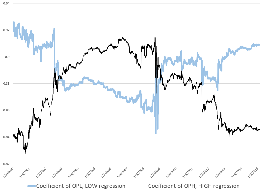
Note the abrupt changes in the values of the coefficients of OPH_t and OPL_t in 2008.

These plausibly reflect stock market volatility in the Great Recession. After 2010 the value of both coefficients tends to move back to levels seen at the beginning of the study period.

This suggests trajectories influenced by the general climate of risk for investors and their risk preferences.

I am increasingly convinced the influence of these so-called proximity variables is based on heuristics such as “buy when the opening price is greater than the previous period high” or “sell, if the opening price is lower than the previous period low.”

Recall, for example, that the coefficient of OPH_t measures the influence of the spread between the opening price and the previous period high on the growth in the daily high price.

The trajectory, shown in the narrow, black line, trends up in the approach to 2007. This may reflect investors’ greater inclination to buy the underlying stocks, when the opening price is above the previous period high. But then the market experiences the crisis of 2008, and investors abruptly back off from their eagerness to respond to this “buy” signal. With onset of the Great Recession, investors become increasingly risk adverse to such “buy” signals, only starting to recover their nerve after 2013.

A parallel interpretation of the trajectory of the coefficient of OPL_t can be developed based on developments 2008-2009.

Time variation of these coefficients also has implications for out-of-sample forecast errors.

Thus, late 2008, when values of the coefficients of both OPH and OPL make almost vertical movements in opposite directions, is the period of maximum out-of-sample forecast errors. Forecast errors for daily highs, for example, reach a maximum of 8 percent in October 2008. This can be compared with typical errors of less than 0.4 percent for out-of-sample forecasts of daily highs with the proximity variable regressions.

Heuristics

Finally, I recall a German forecasting expert discussing heuristics with an example from baseball. I will try to find his name and give him proper credit. By the idea is that an outfielder trying to catch a flyball does not run calculations involving mass, angle, velocity, acceleration, windspeed, and so forth. Instead, basically, an outfielder runs toward the flyball, keeping it at a constant angle in his vision, so that it falls then into his glove at the last second. If the ball starts descending in his vision, as he approaches it, it may fall on the ground before him. If it starts to float higher in his perspective as he runs to get under it, it may soar over him, landing further back int he field.

I wonder whether similar arguments can be advanced for the strategy of buying based or selling based on spreads between the opening price in a period and the high and low prices in a previous period.