Variable Selection Procedures – The LASSO

The LASSO (Least Absolute Shrinkage and Selection Operator) is a method of automatic variable selection which can be used to select predictors X* of a target variable Y from a larger set of potential or candidate predictors X.

Developed in 1996 by Tibshirani, the LASSO formulates curve fitting as a quadratic programming problem, where the objective function penalizes the absolute size of the regression coefficients, based on the value of a tuning parameter λ. In doing so, the LASSO can drive the coefficients of irrelevant variables to zero, thus performing automatic variable selection.

This post features a toy example illustrating tactics in variable selection with the lasso. The post also dicusses the issue of consistency – how we know from a large sample perspective that we are honing in on the true set of predictors when we apply the LASSO.

My take is a two-step approach is often best. The first step is to use the LASSO to identify a subset of potential predictors which are likely to include the best predictors. Then, implement stepwise regression or other standard variable selection procedures to select the final specification, since there is a presumption that the LASSO “over-selects” (Suggested at the end of On Model Selection Consistency of Lasso).

Toy Example

The LASSO penalizes the absolute size of the regression coefficients, based on the value of a tuning parameter λ. When there are many possible predictors, many of which actually exert zero to little influence on a target variable, the lasso can be especially useful in variable selection.

For example, generate a batch of random variables in a 100 by 15 array – representing 100 observations on 15 potential explanatory variables. Mean-center each column. Then, determine coefficient values for these 15 explanatory variables, allowing several to have zero contribution to the dependent variable. Calculate the value of the dependent variable y for each of these 100 cases, adding in a normally distributed error term.

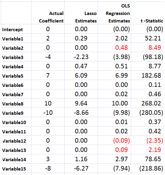
The following Table illustrates something of the power of the lasso.

LassoSS

Using the Matlab lasso procedure and a lambda value of 0.3, seven of the eight zero coefficients are correctly identified. The OLS regression estimate, on the other hand, indicates that three of the zero coefficients are nonzero at a level of 95 percent statistical significance or more (magnitude of the t-statistic > 2).

Of course, the lasso also shrinks the value of the nonzero coefficients. Like ridge regression, then, the lasso introduces bias to parameter estimates, and, indeed, for large enough values of lambda drives all coefficient to zero.

Note OLS can become impossible, when the number of predictors in X* is greater than the number of observations in Y and X. The LASSO, however, has no problem dealing with many predictors.

Real World Examples

For a recent application of the lasso, see the Dallas Federal Reserve occasional paper Hedge Fund Dynamic Market Stability. Note that the lasso is used to identify the key drivers, and other estimation techniques are employed to hone in on the parameter estimates.

For an application of the LASSO to logistic regression in genetics and molecular biology, see Lasso Logistic Regression, GSoft and the Cyclic Coordinate Descent Algorithm, Application to Gene Expression Data. As the title suggests, this illustrates the use of the lasso in logistic regression, frequently utilized in biomedical applications.

Formal Statement of the Problem Solved by the LASSO

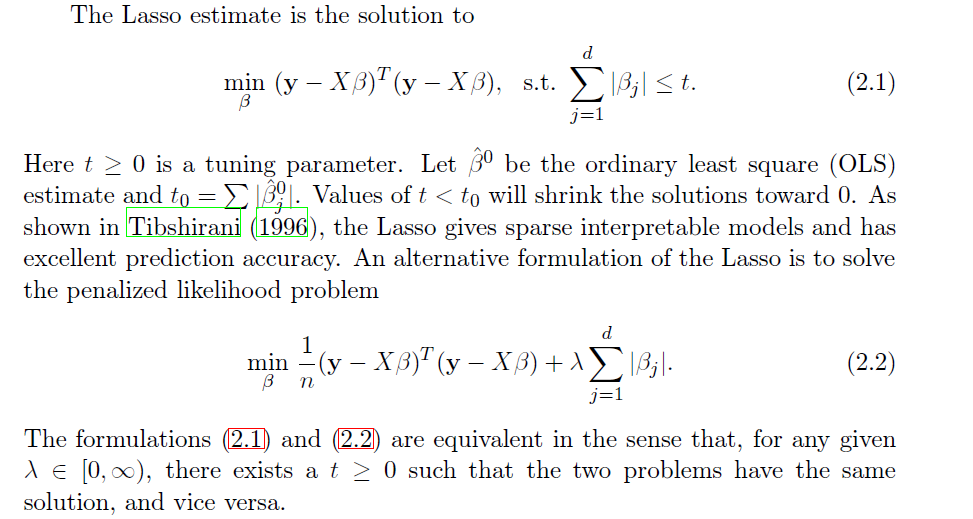
The objective function in the lasso involves minimizing the residual sum of squares, the same entity figuring in ordinary least squares (OLS) regression, subject to a bound on the sum of the absolute value of the coefficients. The following clarifies this in notation, spelling out the objective function.

LassoDerivation

LassoDerivation2

The computation of the lasso solutions is a quadratic programming problem, tackled by standard numerical analysis algorithms. For an analytical discussion of the lasso and other regression shrinkage methods, see the outstanding free textbook The Elements of Statistical Learning by Hastie, Tibshirani, and Friedman.

The Issue of Consistency

The consistency of an estimator or procedure concerns its large sample characteristics. We know the LASSO produces biased parameter estimates, so the relevant consistency is whether the LASSO correctly predicts which variables from a larger set are in fact the predictors.

In other words, when can the LASSO select the “true model?”

Now in the past, this literature is extraordinarily opaque, involving something called the Irrepresentable Condition, which can be glossed as –

almost necessary and sufficient for Lasso to select the true model both in the classical fixed p setting and in the large p setting as the sample size n gets large…This Irrepresentable Condition, which depends mainly on the covariance of the predictor variables, states that Lasso selects the true model consistently if and (almost) only if the predictors that are not in the true model are “irrepresentable” (in a sense to be clarified) by predictors that are in the true model.

Fortunately a ray of light has burst through with Assumptionless Consistency of the Lasso by Chatterjee. Apparently, the LASSO selects the true model almost always – with minimal side assumptions – providing we are satisfied with the prediction error criterion – the mean square prediction error – employed in Tibshirani’s original paper.

Finally, cross-validation is typically used to select the tuning parameter λ, and is another example of this procedure highlighted by Varian’s recent paper.

Geopolitical Risk

USA Today has a headline today What Wall Street is watching in Ukraine crisis and a big red strip across the top of the page with Breaking News Russia issues surrender ultimatum to Ukrainian forces in Crimea.

But the article itself projects calming thoughts, such as,

History also shows that market shocks caused by war, terrorism and other fear-rattling events tend to be short-lived.

In 14 shocks dating back to the attack on Pearl Harbor in December 1941, the median one-day decline has been 2.4%. And the shocks, which also include the Sept. 11 terror attacks and the 1962 Cuban missile crisis, lasted just eight days, with total losses of 7.4%, data from S&P Capital IQ show. The market recouped its losses 14 days later.

Similarly, the Economist February 26 ran an article The return of geopolitical risk noting that,

If there is a consensus, it is probably that geopolitical risks have a tendency to go away. Think back over the last 24 years, going all the way back to the Kuwait crisis, and you will recall that markets sold off initially but recovered as the conflicts turned out either to be shorter, or less economically damaging, than they feared. Hence, while the markets have sold off today, the declines have hardly been substantial (between 0.8% and for the FTSE and 1.4% for the Dax at the time of writing).

Professional organizations in the geopolitical risk space offer to provide information to companies operating in risk-prone areas or with vital interests in, say, natural gas markets globally.

One of these is Stratfor, founded by George Friedman in 1996, with subscription services and reports for purchase by business and other organizations. For the interested, here is a friendly but critical review of Friedman’s supposedly best-selling The Next 100 Years: A Forecast for the 21st Century (2009). Friedman actually predicts the disintegration of Russia in the 2020’s, following a re-assertion of Russian power westward, toward Europe. Hmmm.

Currently, Stratfor is highlighting the potential for the emergence of extreme right-wing groups in the Ukraine. This is a similar focus to one developed in an excellent article in Le Monde Diplomatique Ukraine beyond politics.

I don’t want to comment too extensively on the US role in the Ukraine, or the inevitable saber-rattling and accusations that not enough is being done.

Rather, I think it’s important to look at one particular graphic, presented initially by Business Insider and extensively tweeted thereafter.

Ukrainegas

So from a purely predictive standpoint, it seems unlikely the United States can originate and see implemented significant economic sanctions against Russia – since then, clearly, Russia has the power to retaliate through its control of significant natural gas supplies for western Europe.

The risk – plunging western Europe back into recession, again threatening the US economic recovery.

Economic rationality may provide some constraints to wild responses and actions, but the low performance of many economies since 2009 creates a fertile environment for the emergence of hot-heads, demagogues, and madmen.

So, what I guess I worry about is that the general geopolitical dynamics seem to be moving into greater and greater vulnerability to some idiotic minor event which functions as a tipping point.

But then again, the markets may go forth to a new stabilization very shortly, and it will be business as usual, with more than a modicum of background noise from politics.

Kernel Ridge Regression – A Toy Example

Kernel ridge regression (KRR) is a promising technique in forecasting and other applications, when there are “fat” databases. It’s intrinsically “Big Data” and can accommodate nonlinearity, in addition to many predictors.

Kernel ridge regression, however, is shrouded in mathematical complexity. While this is certainly not window-dressing, it can obscure the fact that the method is no different from ordinary ridge regression on transformations of regressors, except for an algebraic trick to improve computational efficiency.

This post develops a spreadsheet example illustrating this key point – kernel ridge regression is no different from ordinary ridge regression…except for an algebraic trick.

Background

Most applications of KRR have been in the area of machine learning, especially optical character recognition.

To date, the primary forecasting application involves a well-known “fat” macroeconomic database. Using this data, researchers from the Tinbergen Institute and Erasmus University develop KRR models which outperform principal component regressions in out-of-sample forecasts of variables, such as real industrial production and employment.

You might want to tab and review several white papers on applying KRR to business/economic forecasting, including,

Nonlinear Forecasting with Many Predictors using Kernel Ridge Regression

Modelling Issues in Kernel Ridge Regression

Model Selection in Kernel Ridge Regression

This research holds out great promise for KRR, concluding, in one of these selections that,

The empirical application to forecasting four key U.S. macroeconomic variables — production, income, sales, and employment — shows that kernel-based methods are often preferable to, and always competitive with, well-established autoregressive and principal-components-based methods. Kernel techniques also outperform previously proposed extensions of the standard PC-based approach to accommodate nonlinearity.

Calculating a Ridge Regression (and Kernel Ridge Regression)

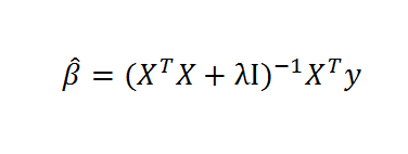
Recall the formula for ridge regression,

aridgeregmatformula                       

Here, X is the data matrix, XT is the transpose of X, λ is the conditioning factor, I is the identify matrix, and y is a vector of values of the dependent or target variable. The “beta-hats” are estimated β’s or coefficient values in the conventional linear regression equation,

y = β1x1+ β2x2+… βNxN

The conditioning factor λ is determined by cross-validation or holdout samples (see Hal Varian’s discussion of this in his recent paper).

Just for the record, ridge regression is a data regularization method which works wonders when there are glitches – such as multicollinearity – which explode the variance of estimated coefficients.

Ridge regression, and kernel ridge regression, also can handle the situation where there are more predictors or explanatory variables than cases or observations.

A Specialized Dataset

Now let us consider ridge regression with the following specialized dataset.

KRRssEx1

By construction, the equation,

y = 2x1 + 5x2+0.25x1x2+0.5x12+1.5x22+0.5x1x22+0.4x12x2+0.2x13+0.3x23

generates the six values of y from the sums of ten terms in x1 and x2, their powers, and cross-products.

Although we really only have two explanatory variables, x1 and x2, the equation, as a sum of 10 terms, can be considered to be constructed out of ten, rather than two, variables.

However, adopting this convenience, it means we have more explanatory variables (10) than observations on the dependent variable (6).

Thus, it will be impossible to estimate the beta’s by OLS.

Of course, we can develop estimates of the values of the coefficients of the true relationship between y and the data on the explanatory variables with ridge regression.

Then, we will find that we can map all ten of these apparent variables in the equation onto a kernel of two variables, simplifying the matrix computations in a fundamental way, using this so-called algebraic trick.

The ordinary ridge regression data matrix X is 6 rows by 10 columns, since there are six observations or cases and ten explanatory variables. Thus, the transpose XT is a 10 by 6 matrix. Accordingly, the product XTX is a 10 by 10 matrix, resulting in a 10 by 10 inverse matrix after the conditioning factor and identity matrix is added in to XTX.

In fact, the matrix equation for ridge regression can be calculated within a spreadsheet using the Excel functions mmult(.,) and minverse() and the transpose operation from Copy. The conditioning factor λ can be determined by trial and error, or by writing a Visual Basic algorithm to explore the mean square error of parameter values associated with different values λ.

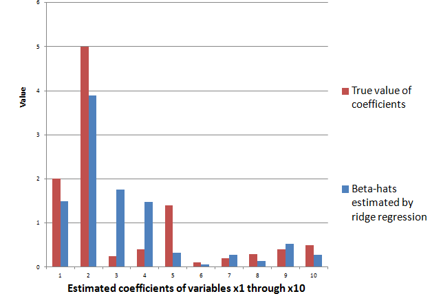
The ridge regression formula above, therefore, gives us estimates for ten beta-hats, as indicated in the following chart, using a λ or conditioning coefficient of .005.

krrbarchart

The red bars indicate the true coefficient values, and the blue bars are the beta-hats estimated by the ridge regression formula.

As you can see, ridge regression “gets in the ballpark” in terms of the true values of the coefficients of this linear expression. However, with only 6 observations, the estimate is highly approximate.

The Kernel Trick

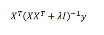
Now with suitable pre- and post-multiplications and resorting, it is possible to switch things around to another matrix formula,

KRRMatformula

Exterkate et al show the matrix algebra in a section of their “Nonlinear..” white paper using somewhat different symbolism.

Key point – the matrix formula listed just above involves inverting a smaller matrix, than the original formula – in our example, a 6 by 6, rather than a 10 by 10 matrix.

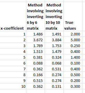
The following Table shows the beta-hats estimated by these two formulas are similar and compares them with the “true” values of the coefficients.

krrcomp

Differences in the estimates by these formally identical formulas relate strictly to issues at the level of numerical analysis and computation.

Kernels

Notice that the ten variables could correspond to a Taylor expansion which might be used to estimate the value of a nonlinear function. This is a key fact and illustrates the concept of a “kernel”.

Thus, designating K = XXT,we find that the elements of K can be obtained without going through the indicated multiplication of these two matrices. This is because K is a polynomial kernel.

There is a great deal more that can be said about this example and the technique in general. Two big areas are (a) arriving at the estimate of the conditioning factor λ and (b) discussing the range of possible kernels that can be used, what makes a kernel a kernel, how to generate kernels from existing kernels, where Hilbert spaces come into the picture, and so forth.

But hopefully this simple example can point the way.

For additional insight and the source for the headline Homer Simpson graphic, see The Kernel Trick.