I’ve been reading about the bootstrap. I’m interested in bagging or bootstrap aggregation.
The primary task of a statistician is to summarize a sample based study and generalize the finding to the parent population in a scientific manner..
The purpose of a sample study is to gather information cheaply in a timely fashion. The idea behind bootstrap is to use the data of a sample study at hand as a “surrogate population”, for the purpose of approximating the sampling distribution of a statistic; i.e. to resample (with replacement) from the sample data at hand and create a large number of “phantom samples” known as bootstrap samples. The sample summary is then computed on each of the bootstrap samples (usually a few thousand). A histogram of the set of these computed values is referred to as the bootstrap distribution of the statistic.
These well-phrased quotes come from Bootstrap: A Statistical Method by Singh and Xie.
OK, so let’s do a simple example.
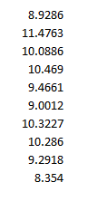
Suppose we generate ten random numbers, drawn independently from a Gaussian or normal distribution with a mean of 10 and standard deviation of 1.
This sample has an average of 9.7684. We would like to somehow project a 95 percent confidence interval around this sample mean, to understand how close it is to the population average.
So we bootstrap this sample, drawing 10,000 samples of ten numbers with replacement.
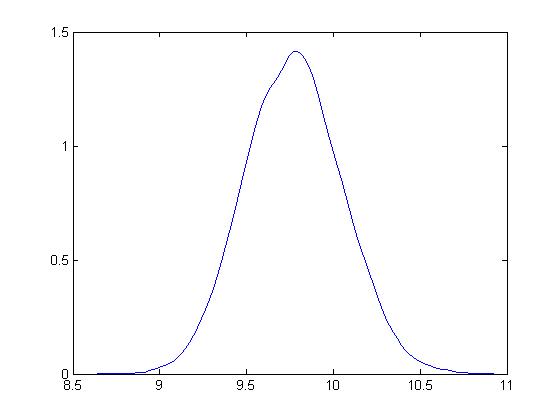
Here is the distribution of bootstrapped means of these samples.
The mean is 9.7713.
Based on the method of percentiles, the 95 percent confidence interval for the sample mean is between 9.32 and 10.23, which, as you note, correctly includes the true mean for the population of 10.
Bias-correction is another primary use of the bootstrap. For techies, there is a great paper from the old Bell Labs called A Real Example That Illustrates Properties of Bootstrap Bias Correction. Unfortunately, you have to pay a fee to the American Statistical Association to read it – I have not found a free copy on the Web.
In any case, all this is interesting and a little amazing, but what we really want to do is look at the bootstrap in developing forecasting models.
Bootstrapping Regressions
There are several methods for using bootstrapping in connection with regressions.
One is illustrated in a blog post from earlier this year. I treated the explanatory variables as variables which have a degree of randomness in them, and resampled the values of the dependent variable and explanatory variables 200 times, finding that doing so “brought up” the coefficient estimates, moving them closer to the underlying actuals used in constructing or simulating them.
This method works nicely with hetereoskedastic errors, as long as there is no autocorrelation.
Another method takes the explanatory variables as fixed, and resamples only the residuals of the regression.
Bootstrapping Time Series Models
The underlying assumptions for the standard bootstrap include independent and random draws.
This can be violated in time series when there are time dependencies.
Of course, it is necessary to transform a nonstationary time series to a stationary series to even consider bootstrapping.
But even with a time series that fluctuates around a constant mean, there can be autocorrelation.
So here is where the block bootstrap can come into play. Let me cite this study – conducted under the auspices of the Cowles Foundation (click on link) – which discusses the asymptotic properties of the block bootstrap and provides key references.
There are many variants, but the basic idea is to sample blocks of a time series, probably overlapping blocks. So if a time series yt has n elements, y1,..,yn and the block length is m, there are n-m blocks, and it is necessary to use n/m of these blocks to construct another time series of length n. Issues arise when m is not a perfect divisor of n, and it is necessary to develop special rules for handling the final values of the simulated series in that case.
Block bootstrapping is used by Bergmeir, Hyndman, and Benıtez in bagging exponential smoothing forecasts.
How Good Are Bootstrapped Estimates?
Consistency in statistics or econometrics involves whether or not an estimate or measure converges to an unbiased value as sample size increases – or basically goes to infinity.
This is a huge question with bootstrapped statistics, and there are new findings all the time.
Interestingly, sometimes bootstrapped estimates can actually converge faster to the appropriate unbiased values than can be achieved simply by increasing sample size.
And some metrics really do not lend themselves to bootstrapping.
Also some samples are inappropriate for bootstrapping. Gelman, for example, writes about the problem of “separation” in a sample –
[In} ..an example of a poll from the 1964 U.S. presidential election campaign, … none of the black respondents in the sample supported the Republican candidate, Barry Goldwater… If zero black respondents in the sample supported Barry Goldwater, then zero black respondents in any bootstrap sample will support Goldwater as well. Indeed, bootstrapping can exacerbate separation by turning near-separation into complete separation for some samples. For example, consider a survey in which only one or two of the black respondents support the Republican candidate. The resulting logistic regression estimate will be noisy but it will be finite.
Here is a video doing a good job of covering the bases on boostrapping. I suggest sampling portions of it first. It’s quite good, but it may seem too much going into it.


