Category Archives: bootstrapping

Global Energy Forecasting Competitions

The 2012 Global Energy Forecasting Competition was organized by an IEEE Working Group to connect academic research and industry practice, promote analytics in engineering education, and prepare for forecasting challenges in the smart grid world. Participation was enhanced by alliance with Kaggle for the load forecasting track. There also was a second track for wind power forecasting.

Hundreds of people and many teams participated.

This year’s April/June issue of the International Journal of Forecasting (IJF) features research from the winners.

Before discussing the 2012 results, note that there’s going to be another competition – the Global Energy Forecasting Competition 2014 – scheduled for launch August 15 of this year. Professor Tao Hong, a key organizer, describes the expansion of scope,

GEFCom2014 (www.gefcom.org) will feature three major upgrades: 1) probabilistic forecasts in the form of predicted quantiles; 2) four tracks on demand, price, wind and solar; 3) rolling forecasts with incremental data update on weekly basis.

Results of the 2012 Competition

The IJF has an open source article on the competition. This features a couple of interesting tables about the methods in the load and wind power tracks (click to enlarge).

hload

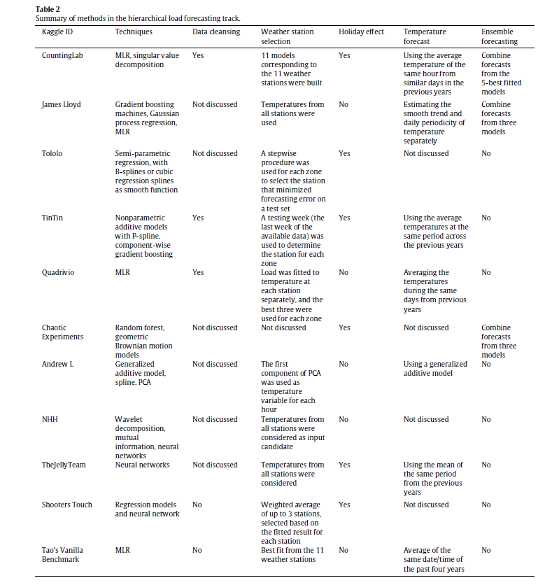
The error metric is WRMSE, standing for weighted root mean square error. One week ahead system (as opposed to zone) forecasts received the greatest weight. The top teams with respect to WRMSE were Quadrivio, CountingLab, James Lloyd, and Tololo (Électricité de France).

wind

The top wind power forecasting teams were Leustagos, DuckTile, and MZ based on overall performance.

Innovations in Electric Power Load Forecasting

The IJF overview article pitches the hierarchical load forecasting problem as follows:

participants were required to backcast and forecast hourly loads (in kW) for a US utility with 20 zones at both the zonal (20 series) and system (sum of the 20 zonal level series) levels, with a total of 21 series. We provided the participants with 4.5 years of hourly load and temperature history data, with eight non-consecutive weeks of load data removed. The backcasting task is to predict the loads of these eight weeks in the history, given actual temperatures, where the participants are permitted to use the entire history to backcast the loads. The forecasting task is to predict the loads for the week immediately after the 4.5 years of history without the actual temperatures or temperature forecasts being given. This is designed to mimic a short term load forecasting job, where the forecaster first builds a model using historical data, then develops the forecasts for the next few days.

One of the top entries is by a team from Électricité de France (EDF) and is written up under the title GEFCom2012: Electric load forecasting and backcasting with semi-parametric models.

This is behind the International Journal of Forecasting paywall at present, but some of the primary techniques can be studied in a slide set by Yannig Goulde.

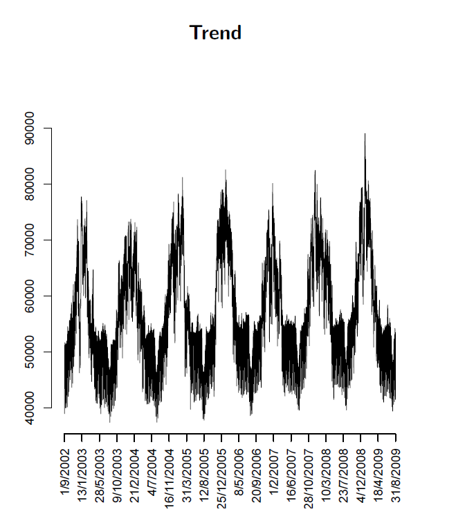
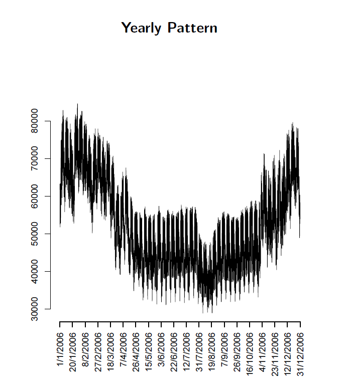
This is an interesting deck because it maps key steps in using semi-parametric models and illustrates real world system power load or demand data, as in this exhibit of annual variation showing the trend over several years.

trend

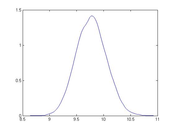
Or this exhibit showing annual variation.

annual

What intrigues me about the EDF approach in the competition and, apparently, more generally in their actual load forecasting, is the use of splines and knots. I’ve seen this basic approach applied in other time series contexts, for example, to facilitate bagging estimates.

So these competitions seem to provide solid results which can be applied in a real-world setting.

Top image from Triple-Curve

Bootstrapping

I’ve been reading about the bootstrap. I’m interested in bagging or bootstrap aggregation.

The primary task of a statistician is to summarize a sample based study and generalize the finding to the parent population in a scientific manner..

The purpose of a sample study is to gather information cheaply in a timely fashion. The idea behind bootstrap is to use the data of a sample study at hand as a “surrogate population”, for the purpose of approximating the sampling distribution of a statistic; i.e. to resample (with replacement) from the sample data at hand and create a large number of “phantom samples” known as bootstrap samples. The sample summary is then computed on each of the bootstrap samples (usually a few thousand). A histogram of the set of these computed values is referred to as the bootstrap distribution of the statistic.

These well-phrased quotes come from Bootstrap: A Statistical Method by Singh and Xie.

OK, so let’s do a simple example.

Suppose we generate ten random numbers, drawn independently from a Gaussian or normal distribution with a mean of 10 and standard deviation of 1.

vector

This sample has an average of 9.7684. We would like to somehow project a 95 percent confidence interval around this sample mean, to understand how close it is to the population average.

So we bootstrap this sample, drawing 10,000 samples of ten numbers with replacement.

Here is the distribution of bootstrapped means of these samples.

bootstrapdist

The mean is 9.7713.

Based on the method of percentiles, the 95 percent confidence interval for the sample mean is between 9.32 and 10.23, which, as you note, correctly includes the true mean for the population of 10.

Bias-correction is another primary use of the bootstrap. For techies, there is a great paper from the old Bell Labs called A Real Example That Illustrates Properties of Bootstrap Bias Correction. Unfortunately, you have to pay a fee to the American Statistical Association to read it – I have not found a free copy on the Web.

In any case, all this is interesting and a little amazing, but what we really want to do is look at the bootstrap in developing forecasting models.

Bootstrapping Regressions

There are several methods for using bootstrapping in connection with regressions.

One is illustrated in a blog post from earlier this year. I treated the explanatory variables as variables which have a degree of randomness in them, and resampled the values of the dependent variable and explanatory variables 200 times, finding that doing so “brought up” the coefficient estimates, moving them closer to the underlying actuals used in constructing or simulating them.

This method works nicely with hetereoskedastic errors, as long as there is no autocorrelation.

Another method takes the explanatory variables as fixed, and resamples only the residuals of the regression.

Bootstrapping Time Series Models

The underlying assumptions for the standard bootstrap include independent and random draws.

This can be violated in time series when there are time dependencies.

Of course, it is necessary to transform a nonstationary time series to a stationary series to even consider bootstrapping.

But even with a time series that fluctuates around a constant mean, there can be autocorrelation.

So here is where the block bootstrap can come into play. Let me cite this study – conducted under the auspices of the Cowles Foundation (click on link) – which discusses the asymptotic properties of the block bootstrap and provides key references.

There are many variants, but the basic idea is to sample blocks of a time series, probably overlapping blocks. So if a time series yt  has n elements, y1,..,yn and the block length is m, there are n-m blocks, and it is necessary to use n/m of these blocks to construct another time series of length n. Issues arise when m is not a perfect divisor of n, and it is necessary to develop special rules for handling the final values of the simulated series in that case.

Block bootstrapping is used by Bergmeir, Hyndman, and Benıtez in bagging exponential smoothing forecasts.

How Good Are Bootstrapped Estimates?

Consistency in statistics or econometrics involves whether or not an estimate or measure converges to an unbiased value as sample size increases – or basically goes to infinity.

This is a huge question with bootstrapped statistics, and there are new findings all the time.

Interestingly, sometimes bootstrapped estimates can actually converge faster to the appropriate unbiased values than can be achieved simply by increasing sample size.

And some metrics really do not lend themselves to bootstrapping.

Also some samples are inappropriate for bootstrapping.  Gelman, for example, writes about the problem of “separation” in a sample

[In} ..an example of a poll from the 1964 U.S. presidential election campaign, … none of the black respondents in the sample supported the Republican candidate, Barry Goldwater… If zero black respondents in the sample supported Barry Goldwater, then zero black respondents in any bootstrap sample will support Goldwater as well. Indeed, bootstrapping can exacerbate separation by turning near-separation into complete separation for some samples. For example, consider a survey in which only one or two of the black respondents support the Republican candidate. The resulting logistic regression estimate will be noisy but it will be finite.

Here is a video doing a good job of covering the bases on boostrapping. I suggest sampling portions of it first. It’s quite good, but it may seem too much going into it.