Category Archives: impact of QE

The End of Quantitative Easing, the Expansion of QE

The US Federal Reserve Bank declared an end to its quantitative easing (QE) program at the end of October.

QE involves direct Fed intervention into buying longer term bonds with an eye to exercising leverage on long term interest rates and, thus, encouraging investment. Readers wanting more detail on how QE is implemented – check Ed Dolan’s slide show Quantitative Easing and the Fed 2008-2014: A Tutorial

The New York Times article on the Fed actions – Quantitative Easing Is Ending. Here’s What It Did, in Charts – had at least two charts that are must-see’s.

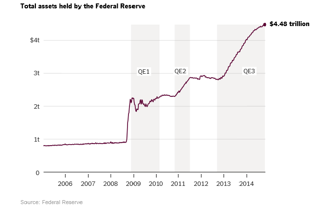
First, the ballooning of the Federal Reserve Balance sheet from less than $1 trillion to $4.5 trillion today –

FedQEassets

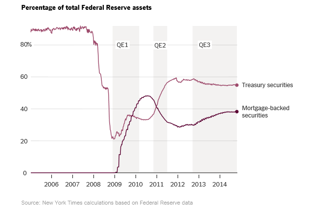
Secondly, according to Times estimates, about 40 percent of Fed assets are comprised of mortgage-backed securities now – making the Fed a potential major player in the US housing markets.

MBS

Several recent articles offer interpretation – what does the end of this five-year long program mean for the US economy and for investors. What were the impacts of QE?

I thought Jeff Miller’s “Old Prof” compendium was especially good – Weighing the Week Ahead: What the End of QE Means for the Individual Investor. If you click this link and find a post more recent than November 1, scroll down for the QE discussion. Basically, Miller thinks the impact on investors will be minimal.

This is also true in the Business Week article The Hawaiian Tropic Effect: Why the Fed’s Quantitative Easing Isn’t Over

But quantitative easing is the gift that keeps on giving. Even after the purchases end, its effects will persist. How could that be? The Fed will still own all those bonds it bought, and according to the agency itself, it’s the level of its holdings that affects the bond market, not the rate of addition to those holdings. Having reduced the supply of bonds available on the market, the Fed has raised their price. Yields (i.e. market interest rates) go down when prices go up. So the effect of quantitative easing is to lower interest rates for things Americans actually care about, such as 30-year fixed-rate mortgages.

Some other articles which attempt to tease out exactly what impacts QE did have on the economy –

Evaluation of quantitative easing QE had “some effects” but it’s one of several influences on the bond market and long term interest rates.

Quantitative easing: giving cash to the public would have been more effective

QE has also had unforeseen side-effects. The policy involved allowing banks and other financial institutions to exchange bonds for cash, and the hope was that this would lead to improved flows of credit to firms looking to expand. In reality, it encouraged financial speculation in property, shares and commodities. The bankers and the hedge fund owners did well out of QE, but the side-effect of footloose money searching the globe for high yields was higher food and fuel prices. High inflation and minimal wage growth led to falling real incomes and a slower recovery.

What Quantitative Easing Did Not Do: Three Revealing Charts – good discussion organized around the following three points –

  1. QE did not work according to the textbook model
  2. QE did not cause inflation
  3. QE was not powerful enough to overcome fiscal restraint

Expansion of QE

But quantitative easing as a central bank policy is by no means a dead letter.

In fact, at the very moment the US Federal Reserve announced the end of its five-year long program of bond-buying, the Bank of Japan (BOPJ) announced a significant expansion of its QE, as noted in this article from Forbes.

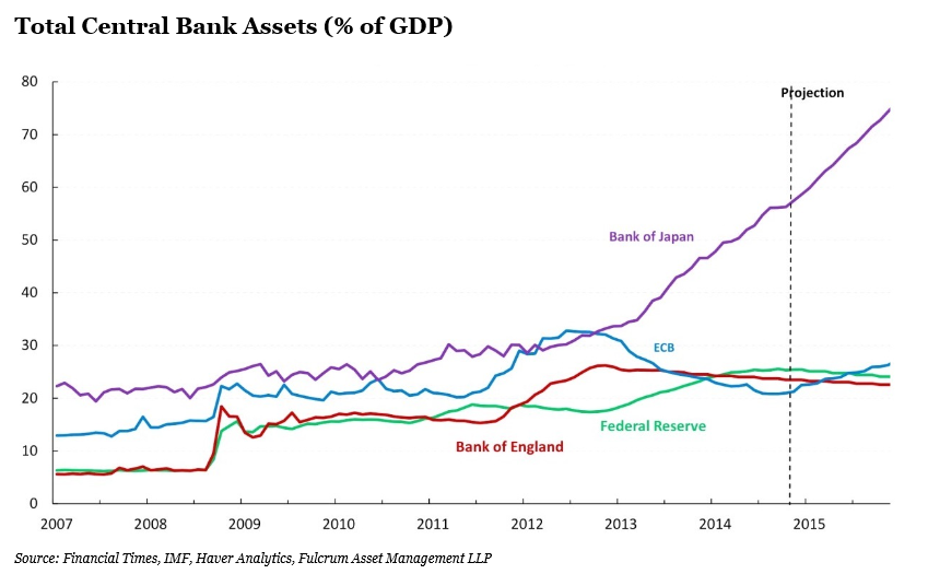
Last week, as the Federal Reserve officially announced the end of its long-term asset purchase program (commonly known as QE3), the Bank of Japan significantly ratcheted up its own quantitative easing program, in a surprising 5-4 split decision. Starting next year, the Bank of Japan will increase its balance sheet by 15 percent of GDP per annum and will extend the average duration of its bond purchases from 7 years to 10 years. The big move by Japan’s central bank comes amid the country’s GDP declining by 7.1% in the second quarter of 2014 (on an annualized basis) from the previous quarter following the increase of the VAT sales tax from 5% to 8% in Japan earlier this year and worries that Japan could fall into another deflationary spiral..

The scale of the Japanese effort is truly staggering, as this chart from the Forbes article illustrates.

 CentralBankAssets

The Economist article on this development Every man for himself tries to work out the implications of the Japanese action on the value of the yen, Japanese inflation/deflation, the Japanese international trade position, impact on competitors (China), and impacts on the US dollar.

What about Europe? Well, Bloomberg offers this primer – Europe’s QE Quandary. Short take – there are 18 nations which have to agree and move together, Germany’s support being decisive. But deflation appears to be spreading in Europe, so many expect something to be done along QE lines.

If you are forecasting for businesses, government agencies, or investors, these developments by central banks around the world are critically important. Their effects may be subtle and largely in unintended consequences, but the scale of operations means you simply have to keep track.

Forecasting Controversies – Impacts of QE

Where there is smoke, there is fire, and other similar adages are suggested by an arcane statistical controversy over quantitative easing (QE) by the US Federal Reserve Bank.

Some say this Fed policy, estimated to have involved $3.7 trillion dollars in asset purchases, has been a bust, a huge waste of money, a give-away program to speculators, but of no real consequence to Main Street.

Others credit QE as the main force behind lower long term interest rates, which have supported US housing markets.

Into the fray jump two elite econometricians – Johnathan Wright of Johns Hopkins and Christopher Neeley, Vice President of the St. Louis Federal Reserve Bank.

The controversy provides an ersatz primer in estimation and forecasting issues with VAR’s (vector autoregressions). I’m not going to draw out all the nuances, but highlight the main features of the argument.

The Effect of QE Announcements From the Fed Are Transitory – Lasting Maybe Two or Three Months

Basically, there is the VAR (vector autoregression) analysis of Johnathan Wright of Johns Hopkins Univeristy, which finds that  –

..stimulative monetary policy shocks lower Treasury and corporate bond yields, but the effects die o¤ fairly fast, with an estimated half-life of about two months.

This is in a paper What does Monetary Policy do to Long-Term Interest Rates at the Zero Lower Bound? made available in PDF format dated May 2012.

More specifically, Wright finds that

Over the period since November 2008, I estimate that monetary policy shocks have a significant effect on ten-year yields and long-maturity corporate bond yields that wear o¤ over the next few months. The effect on two-year Treasury yields is very small. The initial effect on corporate bond yields is a bit more than half as large as the effect on ten-year Treasury yields. This finding is important as it shows that the news about purchases of Treasury securities had effects that were not limited to the Treasury yield curve. That is, the monetary policy shocks not only impacted Treasury rates, but were also transmitted to private yields which have a more direct bearing on economic activity. There is slight evidence of a rotation in breakeven rates from Treasury Inflation Protected Securities (TIPS), with short-term breakevens rising and long-term forward breakevens falling.

Not So, Says A Federal Reserve Vice-President

Christopher Neeley at the St. Louis Federal Reserve argues Wright’s VAR system is unstable and has poor performance in out-of-sample predictions. Hence, Wright’s conclusions cannot be accepted, and, furthermore, that there are good reasons to believe that QE has had longer term impacts than a couple of months, although these become more uncertain at longer horizons.

ChristopherNeely

Neeley’s retort is in a Federal Reserve working paper How Persistent are Monetary Policy Effects at the Zero Lower Bound?

A key passage is the following:

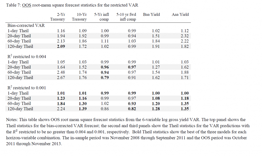
Specifically, although Wright’s VAR forecasts well in sample, it forecasts very poorly out-of-sample and fails structural stability tests. The instability of the VAR coefficients imply that any conclusions about the persistence of shocks are unreliable. In contrast, a naïve, no-change model out-predicts the unrestricted VAR coefficients. This suggests that a high degree of persistence is more plausible than the transience implied by Wright’s VAR. In addition to showing that the VAR system is unstable, this paper argues that transient policy effects are inconsistent with standard thinking about risk-aversion and efficient markets. That is, the transient effects estimated by Wright would create an opportunity for risk-adjusted  expected returns that greatly exceed values that are consistent with plausible risk aversion. Restricted VAR models that are consistent with reasonable risk aversion and rational asset pricing, however, forecast better than unrestricted VAR models and imply a more plausible structure. Even these restricted models, however, do not outperform naïve models OOS. Thus, the evidence supports the view that unconventional monetary policy shocks probably have fairly persistent effects on long yields but we cannot tell exactly how persistent and our uncertainty about the effects of shocks grows with the forecast horizon.

And, it’s telling, probably, that Neeley attempts to replicate Wright’s estimation of a VAR with the same data, checking the parameters, and then conducting additional tests to show that this model cannot be trusted – it’s unstable.

Pretty serious stuff.

Neeley gets some mileage out of research he conducted at the end of the 1990’s in Predictability in International Asset Returns: A Re-examination where he again called into question the longer term forecasting capability of VAR models, given their instabilities.

What is a VAR model?

We really can’t just highlight this controversy without saying a few words about VAR models.

A simple autoregressive relationship for a time series yt can be written as

yt = a1yt-1+..+anyt-n + et

Now if we have other variables (wt, zt..) and we write yt and all these other variables as equations in which the current values of these variables are functions of lagged values of all the variables.

The matrix notation is somewhat hairy, but that is a VAR. It is a system of autoregressive equations, where each variable is expressed as a linear sum of lagged terms of all the other variables.

One of the consequences of setting up a VAR is there are lots of parameters to estimate. So if p lags are important for each of three variables, each equation contains 3p parameters to estimate, so altogether you need to estimate 9p parameters – unless it is reasonable to impose certain restrictions.

Another implication is that there can be reduced form expressions for each of the variables – written only in terms of their own lagged values. This, in turn, suggests construction of impulse-response functions to see how effects propagate down the line.

Additionally, there is a whole history of Bayesian VAR’s, especially associated with the Minneapolis Federal Reserve and the University of Minnesota.

My impression is that, ultimately, VAR’s were big in the 1990’s, but did not live up to their expectations, in terms of macroeconomic forecasting. They gave way after 2000 to the Stock and Watson type of factor models. More variables could be encompassed in factor models than VAR’s, for one thing. Also, factor models often beat the naïve benchmark, while VAR’s frequently did not, at least out-of-sample.

The Naïve Benchmark

The naïve benchmark is a martingale, which often boils down to a simple random walk. The best forecast for the next period value of a martingale is the current period value.

This is the benchmark which Neeley shows the VAR model does not beat, generally speaking, in out-of-sample applications.

Naive

When the ratio is 1 or greater, this means that the mean square forecast error of the VAR is greater than the benchmark model.

Reflections

There are many fascinating details of these papers I am not highlighting. As an old Republican Congressman once said, “a billion here and a billion there, and pretty soon you are spending real money.”

So the defense of QE in this instance boils down to invalidating an analysis which suggests the impacts of QE are transitory, lasting a few months.

There is no proof, however, that QE has imparted lasting impacts on long term interest rates developed in this relatively recent research.