I’ve applied something called loess decomposition to the London PM Fix gold series previously discussed in this blog.

This suggests insights missing from an application of Forecast Pro – a sort of standard in the automatic forecasting field.

Loess decomposition separates a time series into components – trend, seasonals, and residuals or remainder – based on locally weighted regression smoothing of the data.

I always wondered whether, in fact, there was a seasonal component to the monthly London PM fix time series.

Not every monthly or quarterly time series has credible seasonal components, of course.

The proof would seem to be in the pudding. If a program derives seasonal components for a time series, do those seasonal components improve forecasts? That seems to be the critical issue.

STL Decomposition

STL decomposition – seasonal trend decomposition based on loess – was proposed by Cleveland et al in an interesting-sounding publication called “The Journal of Official Statistics.” I found the citation working through the procedure for bagging exponential smoothing mentioned in the previous post.

Amazingly, there is an online resource which calculates this loess decomposition for data you input, based on a listed R routine. The citation is Wessa P., (2013), Decomposition by Loess (v1.0.2) in Free Statistics Software (v1.1.23-r7), Office for Research Development and Education, URL http://www.wessa.net/rwasp_decomposeloess.wasp/

Comparison of STL Decomposition and Forecast Pro Gold Price Forecasts

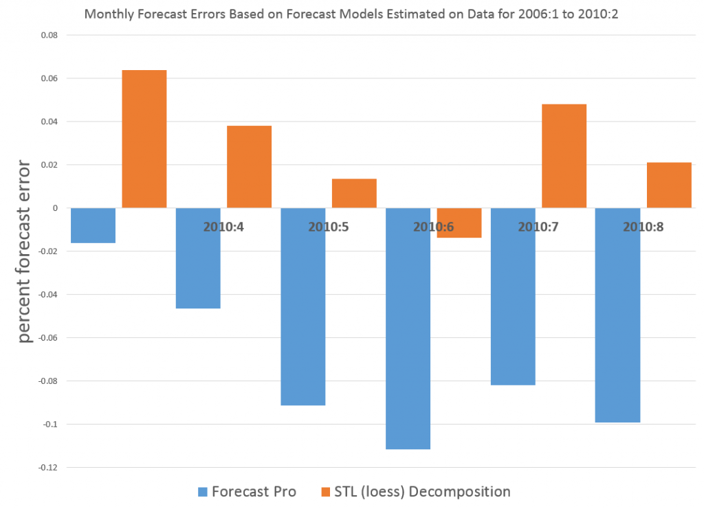
Here’s a typical graph comparing the forecast errors from the Forecast Pro runs with STL Decomposition.

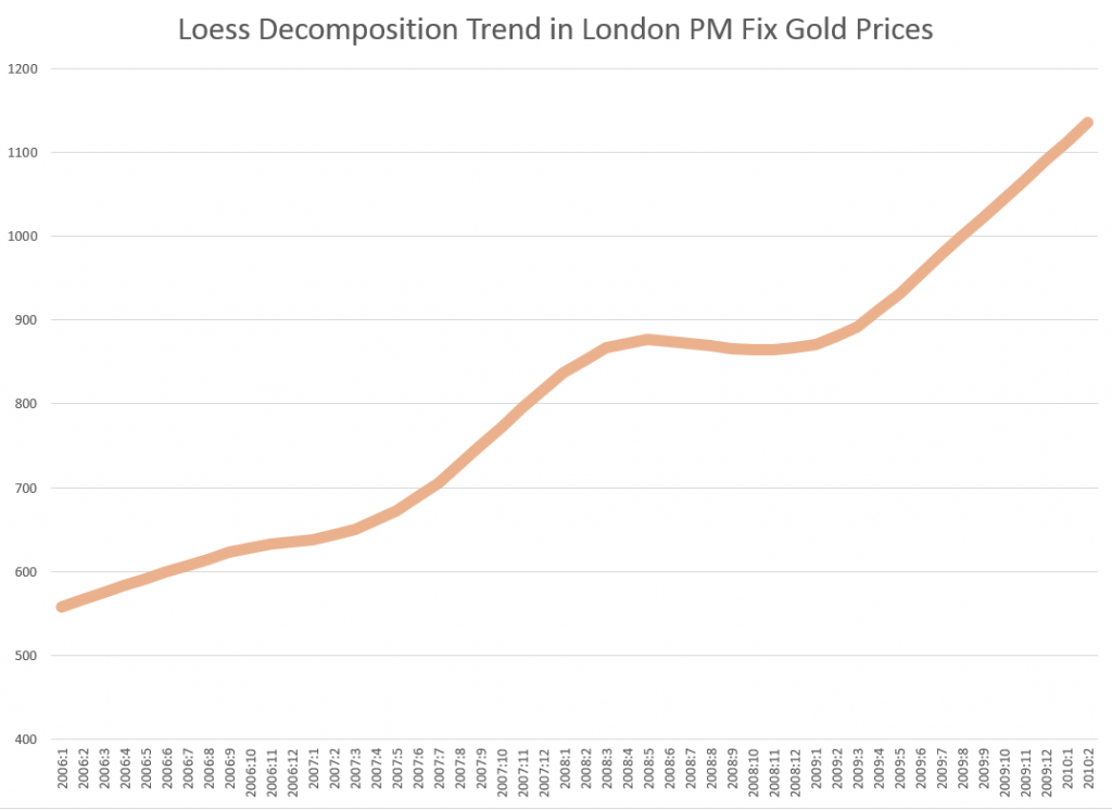
The trend component extracted by the STL decomposition was uncomplicated and easy to forecast by linear extrapolation. I added the seasonal component to these extrapolations to get the monthly forecasts over the six month forecast horizon. Forecast Pro, on the other hand, did not signal the existence of a seasonal component in this series, and, furthermore, identified the optimal forecast model as a random walk and the optimal forecast as the last observed value.

Here is the trend component from the STL decomposition.

Discussion

Potentially, there is lots more to discuss here.

For example, to establish forecasts based on the loess decomposition of the gold price outperform Forecast Pro means compiling a large number of forecast comparisons, ideally one for all possible training sets beyond a minimum number of observations required for stable calculation of the STL algorithm. That is, each training set generates somewhat different values for the trend, seasonals, and residuals with loess decomposition. And Forecast Pro needs to be run for all these possible training sets also, with forecasts compared to out-of-sample data.

While I have not gone to this extent, I have done these computations several times with good results for STL decomposition.

Also, it’s clear that loess decomposition extracts constant variance seasonals. However, the shape of these seasonals change as the training set changes. It is necessary, thus, to study whether these changes can reflect multiplicative seasonality, for series in which that type of seasonality predominates. For example, perhaps STL seasonals tend to reflect the end points of the training sets.

Bergmeir, Hyndman, and Benıtez (BHB) apply a Box Cox transformation in one of their bagged exponential smoothing methods. This is possibly another way to sidestep problems of multiplicative or hetereoskedastic seasonality. It also makes sense when one is attempting to bag a time series.

However, my explorations suggest the results of STL decomposition are quite flexible, and, in the case of this gold price series, often produce superior forecasts to results from one of the main off-the-shelf automatic forecasting programs.

I personally am going to work on including STL decomposition in my forecasting toolkit.