Category Archives: power laws

2014 in Review – I

I’ve been going over past posts, projecting forward my coming topics. I thought I would share some of the best and some of the topics I want to develop.

Recommendations From Early in 2014

I would recommend Forecasting in Data-Limited Situations – A New Day. There, I illustrate the power of bagging to “bring up” the influence of weakly significant predictors with a regression example. This is fairly profound. Weakly significant predictors need not be weak predictors in an absolute sense, providing you can bag the sample to hone in on their values.

There also are several posts on asset bubbles.

Asset Bubbles contains an intriguing chart which proposes a way to “standardize” asset bubbles, highlighting their different phases.

BubbleAnatomy

The data are from the Hong Kong Hang Seng Index, oil prices to refiners (combined), and the NASDAQ 100 Index. I arrange the series so their peak prices – the peak of the bubble – coincide, despite the fact that the peaks occurred at different times (October 2007, August 2008, March 2000, respectively). Including approximately 5 years of prior values of each time series, and scaling the vertical dimensions so the peaks equal 100 percent, suggesting three distinct phases. These might be called the ramp-up, faster-than-exponential growth, and faster-than-exponential decline. Clearly, I am influenced by Didier Sornette in choice of these names.

I’ve also posted several times on climate change, but I think, hands down, the most amazing single item is this clip from “Chasing Ice” showing calving of a Greenland glacier with shards of ice three times taller than the skyscrapers in Lower Manhattan.

See also Possibilities for Abrupt Climate Change.

I’ve been told that Forecasting and Data Analysis – Principal Component Regression is a helpful introduction. Principal component regression is one of the several ways one can approach the problem of “many predictors.”

In terms of slide presentations, the Business Insider presentation on the “Digital Future” is outstanding, commented on in The Future of Digital – I.

Threads I Want to Build On

There are threads from early in the year I want to follow up in Crime Prediction. Just how are these systems continuing to perform?

Another topic I want to build on is in Using Math to Cure Cancer. I’d like to find a sensitive discussion of how MD’s respond to predictive analytics sometime. It seems to me that US physicians are sometimes way behind the curve on what could be possible, if we could merge medical databases and bring some machine learning to bear on diagnosis and treatment.

I am intrigued by the issues in Causal Discovery. You can get the idea from this chart. Here, B → A but A does not cause B – Why?

casualpic

I tried to write an informed post on power laws. The holy grail here is, as Xavier Gabaix says, robust, detail-independent economic laws.

Federal Reserve Policies

Federal Reserve policies are of vital importance to business forecasting. In the past two or three years, I’ve come to understand the Federal Reserve Balance sheet better, available from Treasury Department reports. What stands out is this chart, which anyone surfing finance articles on the net has seen time and again.

FedMBandQEgraph

This shows the total of the “monetary base” dating from the beginning of 2006. The red shaded areas of the graph indicate the time windows in which the various “Quantitative Easing” (QE) policies have been in effect – now three QE’s, QE1, QE2, and QE3.

Obviously, something is going on.

I had fun with this chart in a post called Rhino and Tapers in the Room – Janet Yellen’s Menagerie.

OK, folks, for this intermission, you might want to take a look at Malcolm Gladwell on the 10,000 Hour Rule


So what happens if you immerse yourself in all aspects of the forecasting field?

Coming – how posts in Business Forecast Blog pretty much establish that rational expectations is a concept way past its sell date.

Guy contemplating with wine at top from dreamstime.


Distributions of Stock Returns and Other Asset Prices

This is a kind of wrap-up discussion of probability distributions and daily stock returns.

When I did autoregressive models for daily stock returns, I kept getting this odd, pointy, sharp-peaked distribution of residuals with heavy tails. Recent posts have been about fitting a Laplace distribution to such data.

I have recently been working with the first differences of the logarithm of daily closing prices – an entity the quantitative finance literature frequently calls “daily returns.”

It turns out many researchers have analyzed the distribution of stock returns, finding fundamental similarities in the resulting distributions. There are also similarities for many stocks in many international markets in the distribution of trading volumes and the number of trades. These similarities exist at a range of frequencies – over a few minutes, over trading days, and longer periods.

The paradigmatic distribution of returns looks like this:

NASDAQDR

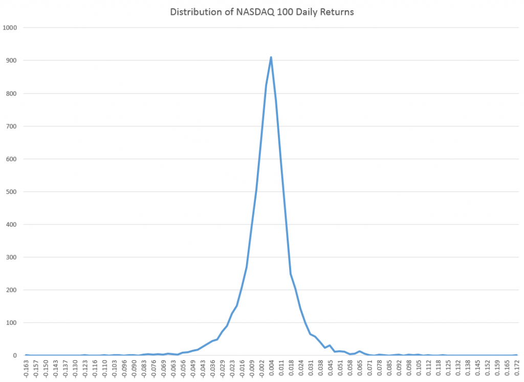
This is based on closing prices of the NASDAQ 100 from October 1985 to the present.

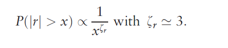
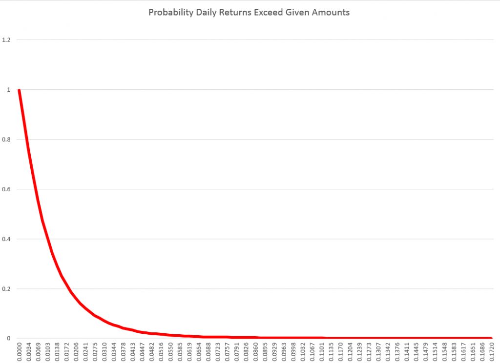
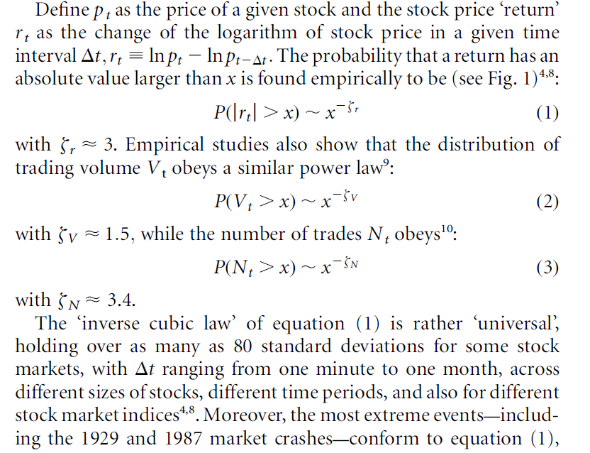
There also are power laws that can be extracted from the probabilities that the absolute value of returns will exceed a certain amount.

For example, again with daily returns from the NASDAQ 100, we get an exponential distribution if we plot these probabilities of exceedance. This curve can be fit by a relationship ~x where θ is between 2.7 and 3.7, depending on where you start the estimation from the top or largest probabilities.

NASDAQABSDR

These magnitudes of the exponent are significant, because they seem to rule out whole classes, such as Levy stable distributions, which require θ < 2.

Also, let me tell you why I am not “extracting the autoregressive components” here. There are probably nonlinear lag effects in these stock price data. So my linear autoregressive equations probably cannot extract all the time dependence that exist in the data. For that reason, and also because it seems pro forma in quantitative finance, my efforts have turned to analyzing what you might call the raw daily returns calculated with price data and suitable transformations.

Levy Stable Distributions

At the turn of the century, Mandelbrot, then Sterling Professor of Mathematics at Yale, wrote an introductory piece for a new journal called Quantitative Finance called Scaling in financial prices: I. Tails and dependence. In that piece, which is strangely convoluted by my lights, Mandelbrot discusses how he began working with Levy-stable distributions in the 1960’s to model the heavy tails of various stock and commodity price returns.

The terminology is a challenge, since there appear to be various ways of discussing so-called stable distributions, which are distributions which yield other distributions of the same type under operations like summing random variables, or taking their ratios.

The Quantitative Finance section of Stack Exchange has a useful Q&A on Levy-stable distributions in this context.

Answers refer readers to Nolan’s 2005 paper Modeling Financial Data With Stable Distributions which tells us that the class of all distributions that are sum-stable is described by four parameters. The distributions controlled by these parameters, however, are generally not accessible as closed algebraic expressions, but must be traced out numerically by computer computations.

Nolan gives several applications, for example, to currency data, illustrated with the following graphs.

Nolan1

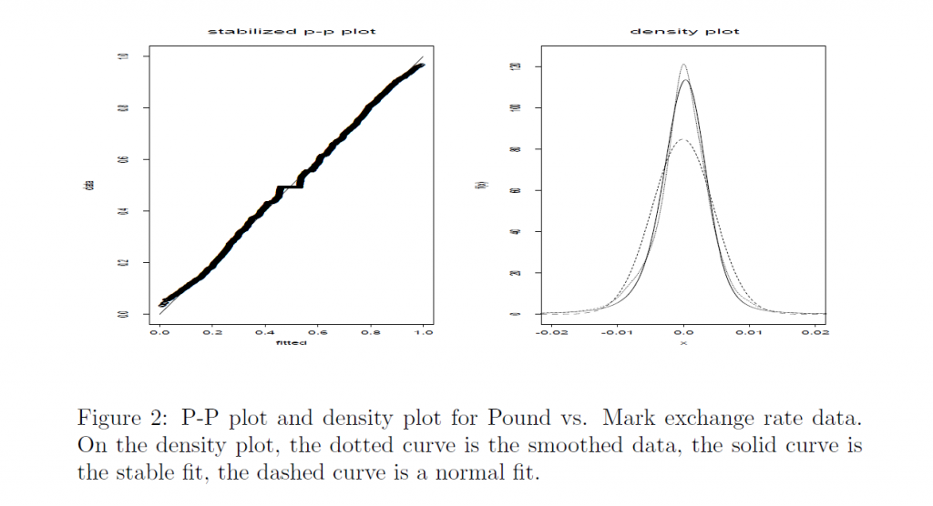
So, the characteristics of the Laplace distribution I find so compelling are replicated to an extent by the Levy-stable distributions.

While Levy-stable distributions continue to be the focus of research in some areas of quantitative finance – risk assessment, for instance – it’s probably true that applications to stock returns are less popular lately. There are two reasons in particular. First, Levy stable distributions apparently have infinite variance, and as Cont writes, there is conclusive evidence that stock prices have finite second moments. Secondly, Levy stable distributions imply power laws for the probability of exceedance of a given level of absolute value of returns, but unfortunately these power laws have an exponent less than 2.

Neither of these “facts” need prove conclusive, though. Various truncated versions of Levy stable distributions have been used in applications like estimating Value at Risk (VAR).

Nolan also maintains a webpage which addresses some of these issues, and provides tools to apply Levy stable distributions.

Why Do These Regularities in Daily Returns and Other Price Data Exist?

If I were to recommend a short list of articles as “must-reads” in this field, Rama Cont’s 2001 survey in Quantitative Finance would be high on the list, as well as Gabraix et al’s 2003 paper on power laws in finance.

Cont provides a list of11 stylized facts regarding the distribution of stock returns.

1. Absence of autocorrelations: (linear) autocorrelations of asset returns are often insignificant, except for very small intraday time scales (

20 minutes) for which microstructure effects come into play.

2. Heavy tails: the (unconditional) distribution of returns seems to display a power-law or Pareto-like tail, with a tail index which is finite, higher than two and less than five for most data sets studied. In particular this excludes stable laws with infinite variance and the normal distribution. However the precise form of the tails is difficult to determine.

3. Gain/loss asymmetry: one observes large drawdowns in stock prices and stock index values but not equally large upward movements.

4. Aggregational Gaussianity: as one increases the time scale t over which returns are calculated, their distribution looks more and more like a normal distribution. In particular, the shape of the distribution is not the same at different time scales.

5. Intermittency: returns display, at any time scale, a high degree of variability. This is quantified by the presence of irregular bursts in time series of a wide variety of volatility estimators.

6. Volatility clustering: different measures of volatility display a positive autocorrelation over several days, which quantifies the fact that high-volatility events tend to cluster in time.

7. Conditional heavy tails: even after correcting returns for volatility clustering (e.g. via GARCH-type models), the residual time series still exhibit heavy tails. However, the tails are less heavy than in the unconditional distribution of returns.

8. Slow decay of autocorrelation in absolute returns: the autocorrelation function of absolute returns decays slowly as a function of the time lag, roughly as a power law with an exponent β ∈ [0.2, 0.4]. This is sometimes interpreted as a sign of long-range dependence.

9. Leverage effect: most measures of volatility of an asset are negatively correlated with the returns of that asset.

10. Volume/volatility correlation: trading volume is correlated with all measures of volatility.

11. Asymmetry in time scales: coarse-grained measures of volatility predict fine-scale volatility better than the other way round.

There’s a huge amount here, and it’s very plainly and well stated.

But then why?

Gabraix et al address this question, in a short paper published in Nature.

Insights into the dynamics of a complex system are often gained by focusing on large fluctuations. For the financial system, huge databases now exist that facilitate the analysis of large fluctuations and the characterization of their statistical behavior. Power laws appear to describe histograms of relevant financial fluctuations, such as fluctuations in stock price, trading volume and the number of trades. Surprisingly, the exponents that characterize these power laws are similar for different types and sizes of markets, for different market trends and even for different countries suggesting that a generic theoretical basis may underlie these phenomena. Here we propose a model, based on a plausible set of assumptions, which provides an explanation for these empirical power laws. Our model is based on the hypothesis that large movements in stock market activity arise from the trades of large participants. Starting from an empirical characterization of the size distribution of those large market participants (mutual funds), we show that the power laws observed in financial data arise when the trading behaviour is performed in an optimal way. Our model additionally explains certain striking empirical regularities that describe the relationship between large fluctuations in prices, trading volume and the number of trades.

The kernel of this paper in Nature is as follows:

powerlaws

Thus, Gabraix links the distribution of purchases in stock and commodity markets with the resulting distribution of daily returns.

I like this hypothesis and see ways it connects with the Laplace distribution and its variants. Probably, I will write more about this in a later post.

Power Laws

Zipf’s Law

George Kingsley Zipf (1902-1950) was an American linguist with degrees from Harvard, who had the distinction of being a University Lecturer – meaning he could give any course at Harvard University he wished to give.

At one point, Zipf hired students to tally words and phrases, showing, in a long enough text, if you count the number of times each word appears, the frequency of words is, up to a scaling constant, 1/n, where n is the rank. So second most frequent word occurs approximately ½ as often as the first; the tenth most frequent word occurs 1/10 as often as the first item, and so forth.

In addition to documenting this relationship between frequency and rank in other languages, including Chinese, Zipf discussed applications to income distribution and other phenomena.

More General Power Laws

Power laws are everywhere in the social, economic, and natural world.

Xavier Gabaix with NYU’s Stern School of Business writes the essence of this subject is the ability to extract a general mathematical law from highly diverse details.

For example, the

..energy that an animal of mass M requires to live is proportional to M3/4. This empirical regularity… has been explained only recently .. along the following lines: If one wants to design an optimal vascular system to send nutrients to the animal, one designs a fractal system, and maximum efficiency exactly delivers the M3/4 law. In explaining the relationship between energy needs and mass, one should not become distracted by thinking about the specific features of animals, such as feathers and fur. Simple and deep principles underlie the regularities.

AnimalMassPL

This type of relationship between variables also characterizes city population and rank, income and wealth distribution, visits to Internet blogs and blog rank, and many other phenomena.

Here is the graph of the power law for city size, developed much earlier by Gabaiux.

CitySizeVSRank

There are many valuable sections in Gabaix’s review article.

However, surely one of the most interesting is the inverse cubic law distribution of stock price fluctuations.

The tail distribution of short-term (15 s to a few days) returns has been analyzed in a series of studies on data sets, with a few thousands of data points (Jansen & de Vries 1991, Lux 1996, Mandelbrot 1963), then with an ever increasing number of data points: Mantegna& Stanley (1995) used 2 million data points, whereas Gopikrishnan et al. (1999) used over 200 million data points. Gopikrishnan et al. (1999) established a strong case for an inverse cubic PL of stock market returns. We let rt denote the logarithmic return over a time interval.. Gopikrishnan et al. (1999) found that the distribution function of returns for the 1000 largest U.S. stocks and several major international indices is

CubicPowerLaw

This relationship holds for positive and negative returns separately.

There is also an inverse half-cubic power law distribution of trading volume.

All this is fascinating, and goes beyond a sort of bestiary of weird social regularities. The holy grail here is, as Gabaix says, robust, detail-independent economic laws.

So with this goal in mind, we don’t object to the intricate details of the aggregation of power laws, or their potential genesis in proportional random growth. I was not aware, for example, that power laws are sustained through additive, multiplicative, min and max operations, possibly explaining why they are so widespread. Nor was I aware that randomly assigning multiplicative growth factors to a group of cities, individuals with wealth, and so forth can generate a power law, when certain noise elements are present.

And Gabaix is also aware that stock market crashes display many attributes that resolve or flow from power laws – so eventually it’s possible general mathematical principles could govern bubble dynamics, for example, somewhat independently of the specific context.

St. Petersburg Paradox

Power laws also crop up in places where standard statistical concepts fail. For example, while the expected or mean earnings from the St. Petersburg paradox coin flipping game does not exist, the probability distribution of payouts follow a power law.

Peter offers to let Paul toss a fair coin an indefinite number of times, paying him 2 coins if it comes up tails on the first toss, 4 coins if the first head comes up on the second toss, and 2n, if the first head comes up on the nth toss.

The paradox is that, with a fair coin, it is possible to earn an indefinitely large payout, depending on how long Paul is willing to flip coins. At the same time, behavioral experiments show that “Paul” is not willing to pay more than a token amount up front to play this game.

The probability distribution function of winnings is described by a power law, so that,

There is a high probability of winning a small amount of money. Sometimes, you get a few TAILS before that first HEAD and so you win much more money, because you win $2 raised to the number of TAILS plus one. Therefore, there is a medium probability of winning a large amount of money. Very infrequently you get a long sequence of TAILS and so you win a huge jackpot. Therefore, there is a very low probability of winning a huge amount of money. These frequent small values, moderately often medium values, and infrequent large values are analogous to the many tiny pieces, some medium sized pieces, and the few large pieces in a fractal object. There is no single average value that is the characteristic value of the winnings per game.

And, as Liebovitch and Scheurle illustrate with Monte Carlo simulations, as more games were played, the average winnings per game of the fractal St. Petersburg coin toss game …increase without bound.

So, neither the expected earnings nor the variance of average earnings exists as computable mathematical entities. And yet the PDF of the earnings is described by the formula Ax-α  where α is near 1.

Closing Thoughts

One reason power laws are so pervasive in the real world is that, mathematically, they aggregate over addition and multiplication. So the sum of two variables described by a power law also is described by a power law, and so forth.

As far as their origin or principle of generation, it seems random proportional growth can explain some of the city size, wealth and income distribution power laws. But I hesitate to sketch the argument, because it seems somehow incomplete, requiring “frictions” or weird departures from a standard limit process.

In any case, I think those of us interested in forecasting should figure ways to integrate these unusual regularities into predictions.