Category Archives: cross-validation

Estimation and Variable Selection with Ridge Regression and the LASSO

I’ve posted on ridge regression and the LASSO (Least Absolute Shrinkage and Selection Operator) some weeks back.

Here I want to compare them in connection with variable selection  where there are more predictors than observations (“many predictors”).

1. Ridge regression does not really select variables in the many predictors situation. Rather, ridge regression “shrinks” all predictor coefficient estimates toward zero, based on the size of the tuning parameter λ. When ordinary least squares (OLS) estimates have high variability, ridge regression estimates of the betas may, in fact, produce lower mean square error (MSE) in prediction.

2. The LASSO, on the other hand, handles estimation in the many predictors framework and performs variable selection. Thus, the LASSO can produce sparse, simpler, more interpretable models than ridge regression, although neither dominates in terms of predictive performance. Both ridge regression and the LASSO can outperform OLS regression in some predictive situations – exploiting the tradeoff between variance and bias in the mean square error.

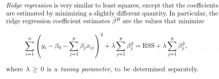
3. Ridge regression and the LASSO both involve penalizing OLS estimates of the betas. How they impose these penalties explains why the LASSO can “zero” out coefficient estimates, while ridge regression just keeps making them smaller. From
An Introduction to Statistical Learning

ridgeregressionOF

Similarly, the objective function for the LASSO procedure is outlined by An Introduction to Statistical Learning, as follows

LASSOobkf

4. Both ridge regression and the LASSO, by imposing a penalty on the regression sum of squares (RWW) shrink the size of the estimated betas. The LASSO, however, can zero out some betas, since it tends to shrink the betas by fixed amounts, as λ increases (up to the zero lower bound). Ridge regression, on the other hand, tends to shrink everything proportionally.

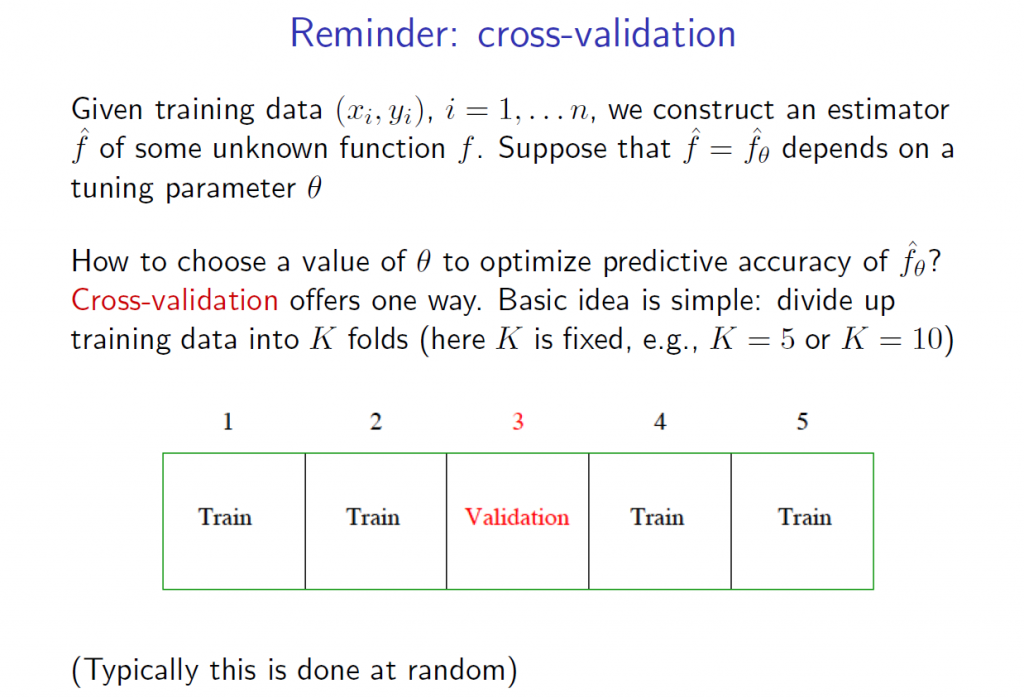
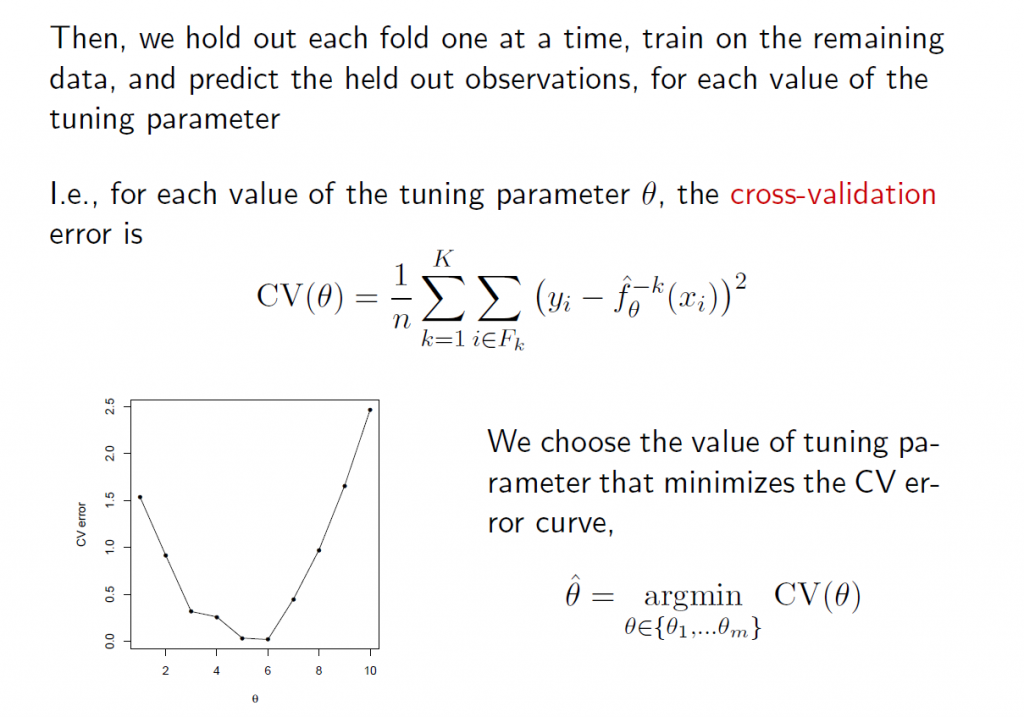
5.The tuning parameter λ in ridge regression and the LASSO usually is determined by cross-validation. Here are a couple of useful slides from Ryan Tibshirani’s Spring 2013 Data Mining course at Carnegie Mellon.

RTCV1

RTCV2

6.There are R programs which estimate ridge regression and lasso models and perform cross validation, recommended by these statisticians from Stanford and Carnegie Mellon. In particular, see glmnet at CRAN. Mathworks MatLab also has routines to do ridge regression and estimate elastic net models.

Here, for example, is R code to estimate the LASSO.

lasso.mod=glmnet(x[train,],y[train],alpha=1,lambda=grid)
plot(lasso.mod)
set.seed(1)
cv.out=cv.glmnet(x[train,],y[train],alpha=1)
plot(cv.out)
bestlam=cv.out$lambda.min
lasso.pred=predict(lasso.mod,s=bestlam,newx=x[test,])
mean((lasso.pred-y.test)^2)
out=glmnet(x,y,alpha=1,lambda=grid)
lasso.coef=predict(out,type=”coefficients”,s=bestlam)[1:20,]
lasso.coef
lasso.coef[lasso.coef!=0]

 What You Get

I’ve estimated quite a number of ridge regression and LASSO models, some with simulated data where you know the answers (see the earlier posts cited initially here) and other models with real data, especially medical or health data.

As a general rule of thumb, An Introduction to Statistical Learning notes,

 ..one might expect the lasso to perform better in a setting where a relatively small number of predictors have substantial coefficients, and the remaining predictors have coefficients that are very small or that equal zero. Ridge regression will perform better when the response is a function of many predictors, all with coefficients of roughly equal size.

The R program glmnet linked above is very flexible, and can accommodate logistic regression, as well as regression with continuous, real-valued dependent variables ranging from negative to positive infinity.

 

First Cut Modeling – All Possible Regressions

If you can, form the regression

Y = β0+ β1X1+ β2X2+…+ βNXN

where Y is the target variable and the N variagles Xi are the predictors which have the highest correlations with the target variables, based on some cutoff value of the correlation, say +/- 0.3.

Of course, if the number of observations you have in the data are less than N, you can’t estimate this OLS regression. Some “many predictors” data shrinkage or dimension reduction technique is then necessary – and will be covered in subsequent posts.

So, for this discussion, assume you have enough data to estimate the above regression.

Chances are that the accompanying measures of significance of the coefficients βi – the t-statistics or standard errors – will indicate that only some of these betas are statistically significant.

And, if you poke around some, you probably will find that it is possible to add some of the predictors which showed low correlation with the target variable and have them be “statistically significant.”

So this is all very confusing. What to do?

Well, if the number of predictors is, say, on the order of 20, you can, with modern computing power, simply calculate all possible regressions with combinations of these 20 predictors. That turns out to be around 1 million regressions (210 – 1). And you can reduce this number by enforcing known constraints on the betas, e.g. increasing family income should be unambiguously related to the target variable and, so, if its sign in a regression is reversed, throw that regression out from consideration.

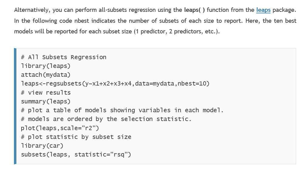
The statistical programming language R has packages set up to do all possible regressions. See, for example, Quick-R which offers this useful suggestion –

leapsBut what other metrics, besides R2, should be used to evaluate the possible regressions?

In-Sample Regression Metrics

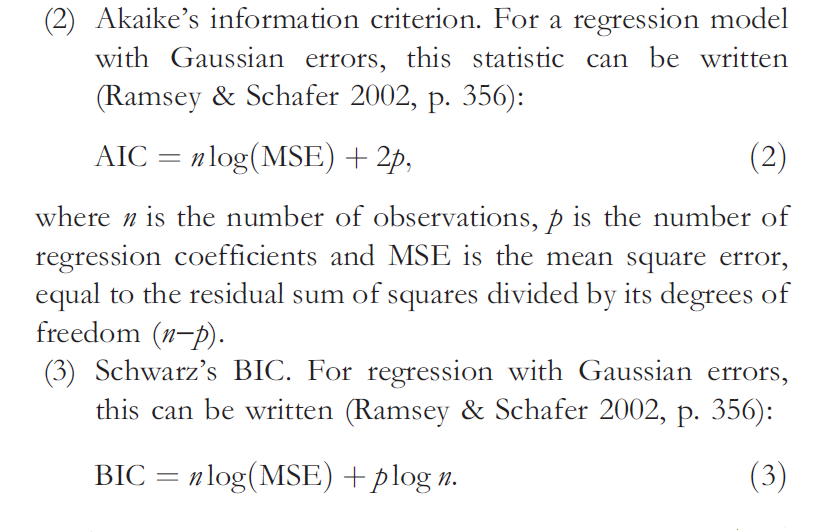
I am not an authority on the Akaike Information Criterion (AIC) or the Bayesian Information Criterion (BIC), which, in addition, to good old R2, are leading in-sample metrics for regression adequacy.

With this disclaimer, here are a few points about the AIC and BIC.

AIC

So, as you can see, both the AIC and BIC are functions of the mean square error (MSE), as well as the number of predictors in the equation and the sample size. Both metrics essentially penalize models with a lot of explanatory variables, compared with other models that might perform similarly with fewer predictors.

  • There is something called the AIC-BIC dilemma. In a valuable reference on variable selection, Serena Ng writes that the AIC is understood to fall short when it comes to consistent model selection. Hyndman, in another must-read on this topic, writes that because of the heavier penalty, the model chosen by BIC is either the same as that chosen by AIC, or one with fewer terms.

Consistency in discussions of regression methods relates to the large sample properties of the metric or procedure in question. Basically, as the sample size n becomes indefinitely large (goes to infinity) consistent estimates or metrics converge to unbiased values. So the AIC is not in every case consistent, although I’ve read research which suggests that the problem only arises in very unusual setups.

  • In many applications, the AIC and BIC can both be minimum for a particular model, suggesting that this model should be given serious consideration.

Out-of-Sample Regression Metrics

I’m all about out-of-sample (OOS) metrics of adequacy of forecasting models.

It’s too easy to over-parameterize models and come up with good testing on in-sample data.

So I have been impressed with endorsements such as that of Hal Varian of cross-validation.

So, ideally, you partition the sample data into training and test samples. You estimate the predictive model on the training sample, and then calculate various metrics of adequacy on the test sample.

The problem is that often you can’t really afford to give up that much data to the test sample.

So cross-validation is one solution.

In k-fold cross validation, you partition the sample into k parts, estimating the designated regression on data from k-1 of those segments, and using the other or kth segment to test the model. Do this k times and then average or somehow collate the various error metrics. That’s the drill.,

Again, Quick-R suggests useful R code.

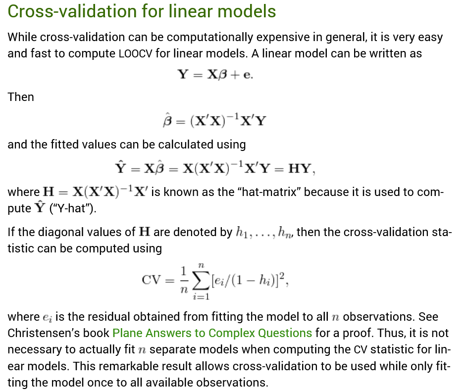
Hyndman also highlights a handy matrix formula to quickly compute the Leave Out One Cross Validation (LOOCV) metric.

LOOCV

LOOCV is not guaranteed to find the true model as the sample size increases, i.e. it is not consistent.

However, k-fold cross-validation can be consistent, if k increases with sample size.

Researchers recently have shown, however, that LOOCV can be consistent for the LASSO.

Selecting regression variables is, indeed, a big topic.

Coming posts will focus on the problem of “many predictors” when the set of predictors is greater in number than the set of observations on the relevant variables.

Top image from Washington Post