Category Archives: business cycle

The Interest Rate Conundrum

It’s time to invoke the parable of the fox and the hedgehog. You know – the hedgehog knows one thing, sees the world through the lens of a single commanding idea, while the fox knows many things, entertains diverse, even conflicting points of view.

This is apropos of my reaction to David Stockman’s The Fed’s Painted Itself Into The Most Dangerous Corner In History—–Why There Will Soon Be A Riot In The Casino.

Stockman, former Director of Office of Management and Budget under President Ronald Reagan who later launched into a volatile career in high finance (See https://en.wikipedia.org/wiki/David_Stockman) currently lends his name to and writes for a spicy website called Contra Corner.

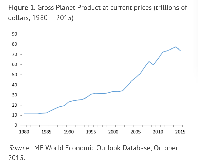
Stockman’s “Why There Will Soon Be a Riot in The Casino” pivots on an Op Ed by Lawrence Summers (Preparing for the next recession) as well as the following somewhat incredible chart, apparently developed from IMF data by Contra Corner researchers.

WEOchart

The storyline is that planetary production fell in current dollar terms in 2015. This isn’t because physical output or hours in service dropped, but because of the precipitous drop in commodity prices and the general pattern of deflation.

All this is apropos of the Fed’s coming decision to raise the federal funds rate from the zero bound (really from about 0.25 percent).

The logic is unassailable. As Summers (former US Treasury Secretary, former President of Harvard, and Professor of Economics at Harvard) writes –

U.S. and international experience suggests that once a recovery is mature, the odds that it will end within two years are about half and that it will end in less than three years are over two-thirds. Because normal growth is now below 2 percent rather than near 3 percent, as has been the case historically, the risk may even be greater now. While the risk of recession may seem remote given recent growth, it bears emphasizing that since World War II, no postwar recession has been predicted a year in advance by the Fed, the White House or the consensus forecast.

But

Historical experience suggests that when recession comes it is necessary to cut interest rates by more than 300 basis points. I agree with the market that the Fed likely will not be able to raise rates by 100 basis points a year without threatening to undermine the recovery. But even if this were possible, the chances are very high that recession will come before there is room to cut rates by enough to offset it. The knowledge that this is the case must surely reduce confidence and inhibit demand.

So let me rephrase this, to underline the points.

  1. Every business recovery has a finite length
  2. The current business recovery has gone on longer than most and probably will end within two or three years
  3. The US Federal Reserve, therefore, has a limited time in which to restore the federal funds rate to something like its historically “normal” levels
  4. But this means a rapid acceleration of interest rates over the next two to three years, something which almost inevitably will speed the onset of a business downturn and which could have alarming global implications
  5. Thus, the Fed probably will not be able to restore the federal funds rate – actually the only rate they directly control – to historically normal values
  6. Therefore, Fed tools to combat the next recession will be severely constrained.
  7. Given these facts and suppositions, secondary speculative/financial and other responses can arise which themselves can become major developments to deal with.

Header pic of fox and hedgehog from willpowered.co.

Economic Outlook – July 2015

For my money, Janet Yellen’s speech July 10 – parts of which I quote below – is important.

Yellen says the Fed plans the first increase in interest rates this year – in September or December, given Fed meeting schedules.

I believe the fact that we have virtually zero interest rates, and have for some time, creates distortions in economic discussions, not to mention its bizarre effects on the real economy.

On the one hand, the US Federal Reserve must realize that if it does not raise interest rates in this phase of the business cycle, it may be a very long time before we get off the zero lower bound. This creates a tendency to “happy talk” from monetary officials, although not Ms. Yellen specifically, papering over weakness in the US and global economy.

On the other hand, I suspect there are now economic interests invested in continuation of low rates, and their contribution going forward may be to sound the alarm at the slightest sign of economic troubles.

And, truly, this expansion phase of the current business cycle is “growing long in the tooth.” It began, according to the National Bureau of Economic Research, in summer 2009. This makes for 96 months from the previous trough of the business cycle to the current time. Only two previous US business expansions historically are longer than this, and only by one or two years.

The price of (economic) freedom is eternal vigilance. With that in mind, consider some of the datapoints on the current economic outlook.

United States

There is an extensive extract from Ms. Yellen’s speech, assessing US economic conditions, the latest report indicating retail sales softened, and the earlier May 2015 consensus forecast of the Survey of Professional Forecasters, indicating lower economic growth expectations.

Janet Yellen’s Speech at the City Club of Cleveland, Ohio

Let me turn now to where I think the economy is headed over the next several years. The latest estimates show that both real GDP and industrial production actually edged down in the first quarter of this year. Some of this weakness appears to be the result of factors that I expect will be only transitory, such as the unusually harsh winter weather in some regions of the country and the West Coast port labor dispute that briefly restrained international trade and caused disruptions in manufacturing supply chains. Also, statistical noise or measurement issues may have played some role. This is not the first time in recent years that real GDP has been reported to decline, or grow unusually slowly, in the first quarter of the year. There is a healthy debate among economists–many within the Federal Reserve System–about some of the technical factors that may lie behind this pattern.4 Nevertheless, at least a couple of other more persistent factors also likely weighed on economic output and industrial production in the first quarter. In particular, the higher foreign exchange value of the dollar that I mentioned, as well as weak growth in some foreign economies, has restrained the demand for U.S. exports. Moreover, lower crude oil prices have significantly depressed business investment in the domestic energy sector. Indeed, industrial production continued to decline somewhat in April and May. We expect the drag on domestic economic activity from these factors to ease over the course of this year, as the value of the dollar and crude oil prices stabilize, and I anticipate moderate economic growth, on balance, for this year as a whole. As always, however, the economic outlook is uncertain. Notably, although the economic recovery in the euro area appears to have gained a firmer footing, the situation in Greece remains unresolved.
JenetYellen

Looking further ahead, I think that many of the fundamental factors underlying U.S. economic activity are solid and should lead to some pickup in the pace of economic growth in the coming years. In particular, I anticipate that employment will continue to expand and the unemployment rate will decline further.

An improving job market should, in turn, help support a faster pace of household spending growth. Additional jobs and potentially faster wage growth bolster household incomes, and lower energy prices mean consumers have more money to spend on other goods and services. In addition, growing employment and wages should make consumers more comfortable in spending a greater portion of their incomes than they have been in the aftermath of the Great Recession. Moreover, increases in house values and stock market prices, along with reductions in debt in recent years, have pushed up households’ net worth, which also should support more spending. Finally, interest rates faced by borrowers remain low, reflecting the FOMC’s highly accommodative monetary policies. Indeed, recent encouraging data about retail sales and light motor vehicle purchases in the beginning of the second quarter could be an indication that the pace of consumer spending is picking up.

Another positive factor for the outlook is that the drag on economic growth in recent years from changes in federal fiscal policies appears to have waned. Temporary fiscal stimulus measures supported economic output during the recession and early in the recovery, but those stimulus measures have since expired, and additional policy actions were taken to reduce the federal budget deficit. By 2011, these changes in fiscal policies were holding back economic growth. However, the effects of those fiscal policy actions now seem to be mostly behind us.5

There are a couple of factors, however, that I expect could restrain economic growth. First, business owners and managers remain cautious and have not substantially increased their capital expenditures despite the solid fundamentals and brighter prospects for consumer spending. Businesses are holding large amounts of cash on their balance sheets, which may suggest that greater risk aversion is playing a role. Indeed, some economic analysis suggests that uncertainty about the strength of the recovery and about government economic policies could be contributing to the restraint in business investment.6

A second factor that could restrain economic growth regards housing. While national home prices have been rising for a few years and home sales have improved recently, residential construction has remained quite soft. Many households still find it difficult to obtain mortgage credit, but, more generally, the weak job market and slow wage gains in recent years appear to have induced people to double-up on housing. For example, many young adults continue to live with their parents. Population growth is creating a need for more housing, whether to rent or to own, and I do expect that continuing job and wage gains will encourage more people to form new households. Nevertheless, activity in the housing sector seems likely to improve only gradually.

Regarding inflation, as I mentioned earlier, the recent effects of lower prices for crude oil and for imports on overall inflation are expected to wane during this year. Combined with further tightening in labor and product markets, I expect inflation will move toward the FOMC’s 2 percent objective over the next few years. Importantly, a number of different surveys indicate that longer-term inflation expectations have remained stable even as recent readings on inflation have fallen. If inflation expectations had not remained stable, I would be more concerned because consumer and business expectations about inflation can become self-fulfilling.

From the New York Times – To my ears, most of Ms. Yellen’s speech expertly laid out why the economy is not ready for interest rate increases anytime soon. Then, toward the end, she said that based on her views, she expected to begin raising rates “at some point later this year.” That would mean a rate hike in three months, at the Fed’s next meeting in September, or six months hence at its December meeting.

ADVANCE MONTHLY SALES FOR RETAIL AND FOOD SERVICES

The U.S. Census Bureau announced today that advance estimates of U.S. retail and food services sales for June, adjusted for seasonal variation and holiday and trading-day differences, but not for price changes, were $442.0 billion, a decrease of 0.3 percent (±0.5%)* from the previous month, but up 1.4 percent (±0.9%) above June 2014. Total sales for the April 2015 through June 2015 period were up 1.7 percent (±0.7%) from the same period a year ago. The April 2015 to May 2015 percent change was revised from +1.2 percent (±0.5%) to +1.0 percent (±0.3%).

Retail trade sales were down 0.3 percent (±0.5%)* from May 2015, but up 0.6 percent (±0.7%)* above last year. Food services and drinking places were up 7.7 percent (±3.3%) from June 2014 and sporting goods, hobby, books and music were up 6.6 percent (±1.9%) from last year. Gasoline stations were down 17.1% (±1.4%) from the previous year.

Second Quarter 2015 Survey of Professional Forecasters

(Release Date: May 15, 2015) Weaker Outlook for Growth

The outlook for growth in the U.S. economy over the next three years looks weaker now than it did in February, according to 44 forecasters surveyed by the Federal Reserve Bank of Philadelphia. The forecasters predict real GDP will grow at an annual rate of 2.5 percent this quarter and 3.1 percent next quarter. On an annual-average over annual-average basis, real GDP will grow 2.4 percent in 2015, down 0.8 percentage point from the previous estimate. The forecasters predict real GDP will grow 2.8 percent each in 2016 and 2017, and 2.5 percent in 2018.

Global

Emerging markets made up some of the slack in the global economy after 2008-2009, but today are everywhere slowing, as the latest revision of the International Monetary Fund (IMF) World Economic Outlook indicates.

IMF July World Economic Outlook – Slower Growth in Emerging Markets, a Gradual Pickup in Advanced Economies

Global growth is projected at 3.3 percent in 2015, marginally lower than in 2014, with a gradual pickup in advanced economies and a slowdown in emerging market and developing economies. In 2016, growth is expected to strengthen to 3.8 percent.

  • A setback to activity in the first quarter of 2015, mostly in North America, has resulted in a small downward revision to global growth for 2015 relative to the April 2015 World Economic Outlook (WEO). Nevertheless, the underlying drivers for a gradual acceleration in economic activity in advanced economies—easy financial conditions, more neutral fiscal policy in the euro area, lower fuel prices, and improving confidence and labor market conditions—remain intact.
  • In emerging market economies, the continued growth slowdown reflects several factors, including lower commodity prices and tighter external financial conditions, structural bottlenecks, rebalancing in China, and economic distress related to geopolitical factors. A rebound in activity in a number of distressed economies is expected to result in a pickup in growth in 2016.
  • The distribution of risks to global economic activity is still tilted to the downside. Near-term risks include increased financial market volatility and disruptive asset price shifts, while lower potential output growth remains an important medium-term risk in both advanced and emerging market economies. Lower commodity prices also pose risks to the outlook in low-income developing economies after many years of strong growth.

Link to Blanchard video

China May Tip World Into Recession: Morgan Stanley

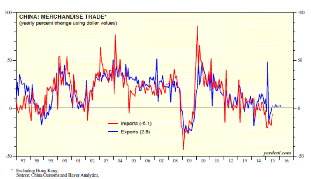
Also there is this interesting chart From Dr. Ed’s Blog
ChinaTrade

Impending Disaster In Greece

My take is that the harsh dealing with Greece led by, apparently, the Germans is more symbolic than directly material to global economic conditions. Nevertheless, it is an ugly symbol, representing, it seems, the end of dreamy thoughts about European integration and the onset of recognition of new German hegemony in Europe.

I am an admirer of modern Germany, having struggled to relearn enough German to read newspapers recently and ask for items in German bakeries. I see the German perspective, but I deeply regret its narrow scope. I think more conservative Germans are missing the big picture here. Of course, the plight of the Greeks is desperate and lamentable.

One final remark – forecasting comes to the fore at junctures such as these. Are we on the cusp, have we started to slide down, or is there still some upside? Compelling questions.

The Holy Grail of Business Forecasting – Forecasting the Next Downturn

What if you could predict the Chicago Fed National Activity Index (CFNAI), interpolated monthly values of the growth of nominal GDP, the Aruoba-Diebold-Scotti (ADS) Business Conditions Index, and the Kansas City Financial Stress Index (KCFSI) three, five, seven, even twelve months into the future? What if your model also predicted turning points in these US indexes, and also similar macroeconomic variables for countries in Asia and the European Union? And what if you could do all this with data on monthly returns on the stock prices of companies in the financial sector?

That’s the claim of Linda Allen, Turan Bali, and Yi Tang in a fascinating 2012 paper Does Systemic Risk in the Financial Sector Predict Future Economic Downturns?

I’m going to refer to these authors as Bali et al, since it appears that Turan Bali, shown below, did some of the ground-breaking research on estimating parametric distributions of extreme losses. Bali also is the corresponding author.

T_bali

Bali et al develop a new macroindex of systemic risk that predicts future real economic downturns which they call CATFIN.

CATFIN is estimated using both value-at-risk (VaR) and expected shortfall (ES) methodologies, each of which are estimated using three approaches: one nonparametric and two different parametric specifications. All data used to construct the CATFIN measure are available at each point in time (monthly, in our analysis), and we utilize an out-of-sample forecasting methodology. We find that all versions of CATFIN are predictive of future real economic downturns as measured by gross domestic product (GDP), industrial production, the unemployment rate, and an index of eighty-five existing monthly economic indicators (the Chicago Fed National Activity Index, CFNAI), as well as other measures of real macroeconomic activity (e.g., NBER recession periods and the Aruoba-Diebold-Scott [ADS] business conditions index maintained by the Philadelphia Fed). Consistent with an extensive body of literature linking the real and financial sectors of the economy, we find that CATFIN forecasts aggregate bank lending activity.

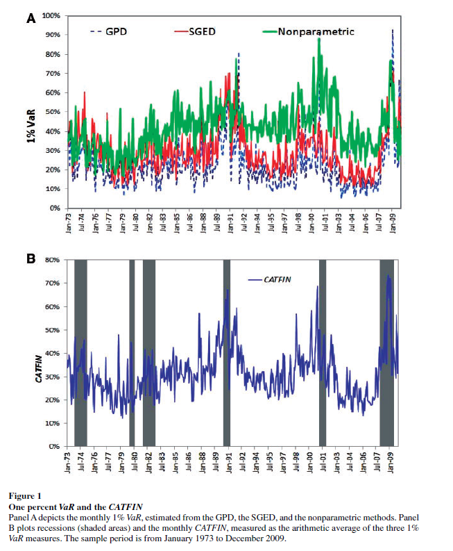
The following graphic illustrates three components of CATFIN and the simple arithmetic average, compared with US recession periods.

CATFIN

Thoughts on the Method

OK, here’s the simple explanation. First, these researchers identify US financial companies based on definitions in Kenneth French’s site at the Tuck School of Business (Dartmouth). There are apparently 500-1000 of these companies for the period 1973-2009. Then, for each month in this period, rates of return of the stock prices of these companies are calculated. Then, three methods are used to estimate 1% value at risk (VaR) – two parametric methods and one nonparametric methods. The nonparametric method is straight-forward –

The nonparametric approach to estimating VaR is based on analysis of the left tail of the empirical return distribution conducted without imposing any restrictions on the moments of the underlying density…. Assuming that we have 900 financial firms in month t , the nonparametric measure of1%VaR is the ninth lowest observation in the cross-section of excess returns. For each month, we determine the one percentile of the cross-section of excess returns on financial firms and obtain an aggregate 1% VaR measure of the financial system for the period 1973–2009.

So far, so good. This gives us the data for the graphic shown above.

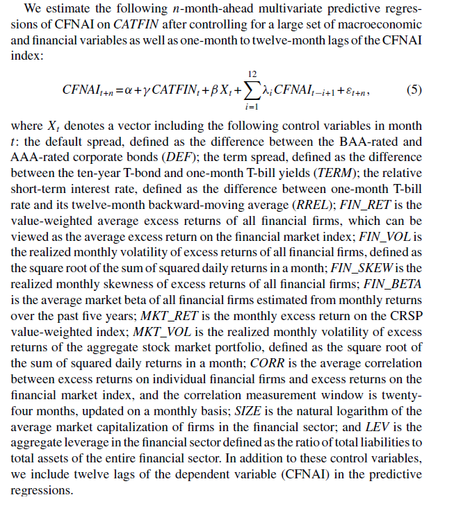
In order to make this predictive, the authors write that –

CATFINEQ

Like a lot of leading indicators, the CATFIN predictive setup “over-predicts” to some extent. Thus, there are there are five instances in which a spike in CATFIN is not followed by a recession, thereby providing a false positive signal of future real economic distress. However, the authors note that in many of these cases, predicted macroeconomic declines may have been averted by prompt policy intervention. Their discussion of this is very interesting, and plausible.

What This Means

The implications of this research are fairly profound – indicating, above all, the priority of the finance sector in leading the overall economy today. Certainly, this consistent with the balance sheet recession of 2008-2009, and probably will continue to be relevant going forward – since nothing really has changed and more concentration of ownership in finance has followed 2008-2009.

I do think that Serena Ng’s basic point in a recent review article probably is relevant – that not all recessions are the same. So it may be that this method would not work as well for, say, the period 1945-1970, before financialization of the US and global economies.

The incredibly ornate mathematics of modeling the tails of return distributions are relevant in this context, incidentally, since the nonparametric approach of looking at the empirical distributions month-by-month could be suspect because of “cherry-picking.” So some companies could be included, others excluded to make the numbers come out. This is much difficult in a complex maximum likelihood estimation process for the location parameters of these obscure distributions.

So the question on everybody’s mind is – WHAT DOES THE CATFIN MODEL INDICATE NOW ABOUT THE NEXT FEW MONTHS? Unfortunately, I am unable to answer that, although I have corresponded with some of the authors to inquire whether any research along such lines can be cited.

Bottom line – very impressive research and another example of how important science can get lost in the dance of prestige and names.

Random Cycles

In 1927, the Russian statistician Eugen Slutsky wrote a classic article called ‘The summation of random causes as the source of cyclic processes,’ a short summary of which is provided by Barnett

If the variables that were taken to represent business cycles were moving averages of past determining quantities that were not serially correlated – either real-world moving averages or artificially generated moving averages – then the variables of interest would become serially correlated, and this process would produce a periodicity approaching that of sine waves

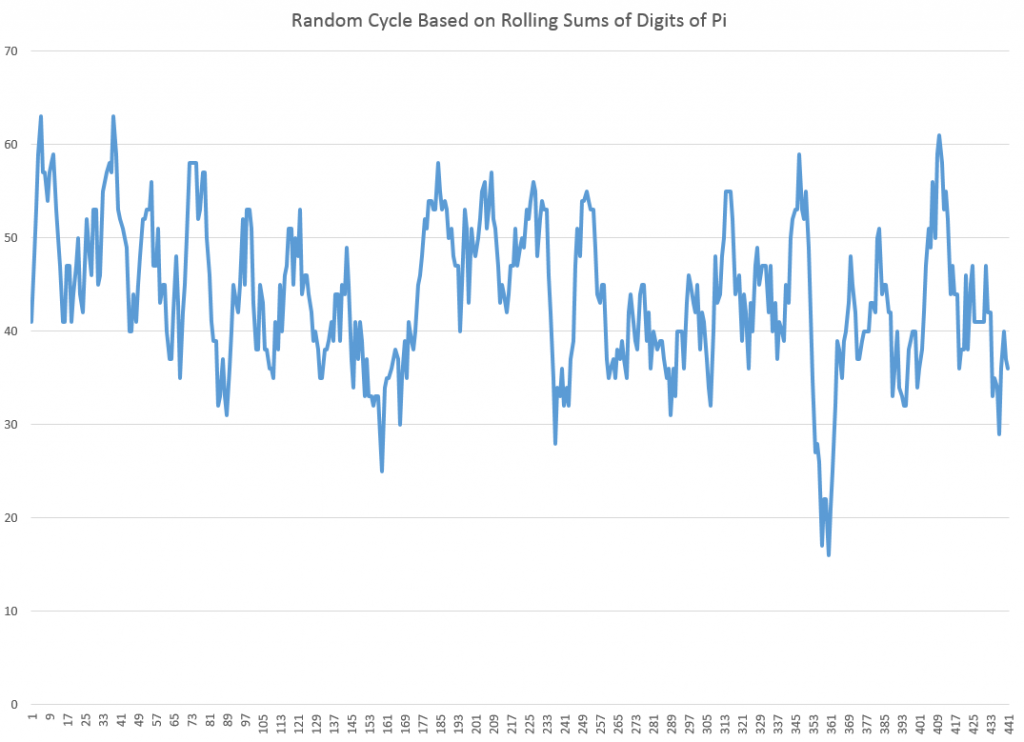
It’s possible to illustrate this phenomena with rolling sums of the digits of pi (π). The following chart illustrates the wave-like result of charting rolling sums of ten consecutive digits of pi.

picycle

So to be explicit, I downloaded the first 450 digits of pi, took them apart, and then graphed the first 440 rolling sums.

The wave-like pattern Illustrates a random cycle.

Forecasting Random Cycles

If we consider this as a time series, each element xk is the following sum,

xk = dk+dk-1+..+dk-10

where dj is the jth digit in the decimal expansion of pi to the right of the initial value of 3.

Now, apparently, it is not proven that the digits of pi are truly random, although one can show that, so far as we can compute, these digits are described by a uniform distribution.

As far as we know, the probability that the next digit will be any digit from 0 to 9 is 1/10=0.1

So as one moves through the digits of pi, generating rolling sums, each new sum means the addition of a new digit, which is unknown and can only be predicted up to its probability. And, at the same time, a digit at the beginning of the preceding sum drops away in the new sum.

Note also that we can always deduce what the series of original digits is, given a series of these rolling sums up to some point.

So the issue is whether the new digit added to the next sum is greater than, equal to, or less than the leading digit of the current sum – which is where we now stand in this sort of analysis. This determines whether the next rolling sum will be greater than, equal to, or less than the current sum.

Here’s where the forecasts can be produced. If the rolling sum is large enough, approaching or equal to 90, there is a high probability that the next rolling sum will be lower, leading to this wave-like pattern. Conversely, if the rolling sum is near zero, the chances are the subsequent sum will be larger. And all this arm-waving can be complemented by exact probabilistic calculations.

Some Ultimate Thoughts

It’s interesting we are really dealing here with a random cycle. That’s proven by the fact that, at any time, the series could go flat-line or trace out some other kind of weird movement.

Thus, the quasi-periodic aspect can be violated for as many periods as you might choose, if one arrives at a run of the same digit in the expansion of pi.

This reminds me of something George Gamow wrote in one of his popular books, where he discusses thermodynamics and the random movement of atoms and molecules in the air of a room. Gamow observes it is entirely possible all the air by chance will congregate in one corner, leaving a vacuum elsewhere. Of course, this is highly improbable.

The only difference would be that there are a finite number of atoms and molecules in the air of any room, but, presumably, an infinite number of digits in the expansion of pi.

The morale of the story is, in any case, to be cautious in imposing a fixed cycle on this type of series.

The Business Cycle

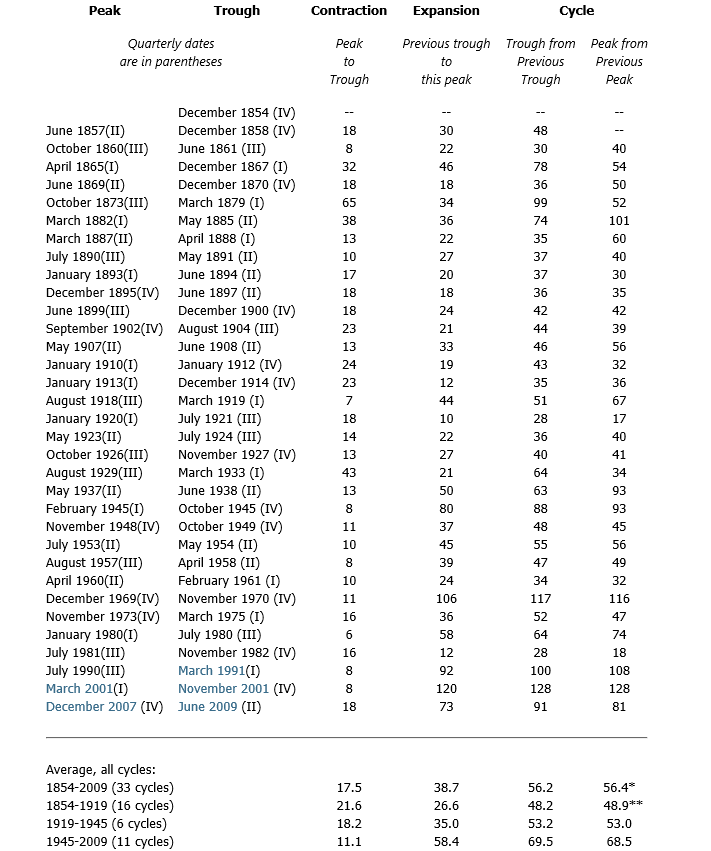
The National Bureau of Economic Research (NBER) has a standing committee which designates the start and finish of recessions, or more precisely, the dates of the peaks and troughs of the US business cycle.

And the NBER site maintains a complete record of the US business cycle, dating back to the middle 1800’s, as shown in the following tables.

NBERbsdates

Periods of contraction, from peak to trough, are typically shorter than periods of expansion – or the movement from previous trough to the next peak.

Since World War II, the average length of the business cycle, variously measured from trough to trough or from peak to peak, is more than 5 years.

Focusing on the current situation, we are interested in the length of time from the previous peak of the business cycle in December 2007 to the next peak. The longest peak to peak period was over the prosperity of the 1990’s, and lasted more than 10 years (128 months).

So, it would be unusual if the peak of this current business cycle were much later than 2017-2018.

In terms of predicting turning points, matters are complicated by the fact that, unlike many European countries, the NBER does not define a recession in terms of two consecutive quarters of decline in real GDP.

Rather, a recession is a significant decline in economic activity spread across the economy, lasting more than a few months, normally visible in real GDP, real income, employment, industrial production, and wholesale-retail sales.

But just predicting the onset of two consecutive quarters of decline in real GDP is challenging. Indeed, the record of macroeconomic forecasting is very poor in this regard.

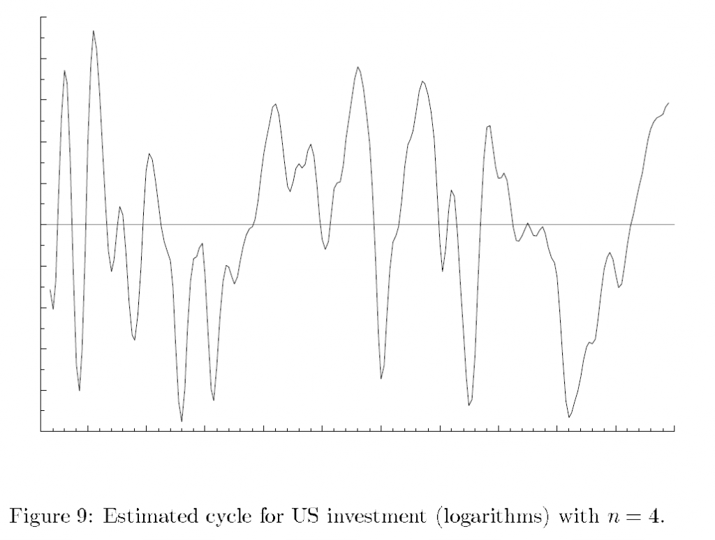
Part of the problem with the concept of a “cycle” in this context is the irregularity of the fluctuations derived by standard filters and methods.

Harvey, for example, applies low band and pass Butterworth filters to US total investment and other macroeconomic series, deriving, at one pont, an investment “cycle” that looks like this.

Invcycle

So almost everything that makes a cycle useful in prediction is missing from this investment cycle. Thus, one cannot conclude that a turning point will occur, when the amplitude of the cycle is reached, since the amplitudes of these quasi-cycles vary considerably. Similarly, the “period” of the cycle is by no means fixed, but is basically stochastic, with a certain variance sometimes expressed as a “hyperparameter.” Only a certain quality of smoothness presents itself, and, of course, is a result of the filtering parameters that are applied.

In my opinion, industry cycles make a certain amount of sense, for particular industries, over particular spans of time. What I mean is that identification of such industry cycles improves predictability of the underlying series – be it sales or inventories or what have you.

The business cycle, on the other hand, is something of a metaphor, or maybe just an evocative phrase.

True, there are periods of economic contraction and periods of expansion.

But the extraction of macroeconomic cycles often does not improve predictability, because the fluctuations so identified are highly irregular from a number of different viewpoints.

I’ve sort of confirmed this is a quantitative sense by applying various cycle-extraction softwares to US real GDP to see whether any product or approach gave a hint that the Great Recession which began in 2008 would (a) occur, and (b) be as dramatic as it was. So far, no go.

And, of course, Ng points out that the Great Recession was fundamentally different than, say, recessions in the 1960’s sand 1970’s in that it was a balance sheet recession.

The Consumer Durable Inventory Cycle – Canary in the Coal Mine?

I’m continuing this week with posts about cycles and, inevitably, need to address one very popular method of extracting cycles from time series data – the Hodrick-Prescott (HP) filter.

Recently, I’ve been exploring inventory cycles, hoping to post something coherent.

I think I hit paydirt, as they say in gold mining circles.

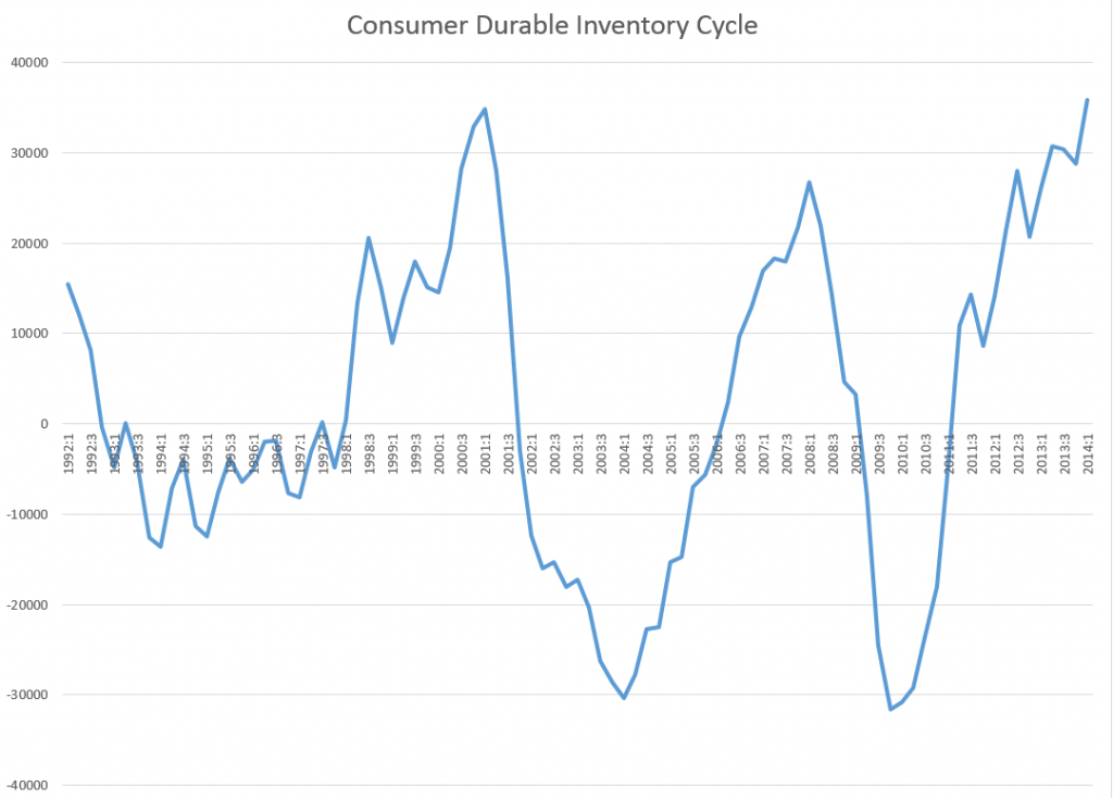
Here is the cycle component extracted from consumer durable inventories (not seasonally adjusted) from the Census manufacturing with a Hodrick-Prescott filter. I use a Matlab implementation here called hpfilter.

CDcycle

In terms of mechanics, the HP filter extracts the trend and cyclical component from a time series by minimizing an expression, as described by Wikipedia –

HPexp

What’s particularly interesting to me is that the peak of the two cycles in the diagram are spot-on the points at which the business cycle goes into recession – in 2001 and 2008.

Not only that, but the current consumer durable inventory cycle is credibly peaking right now and, based on these patterns, should go into a downward movement soon.

Of course, amplitudes of these cycles are a little iffy.

But the existence of a consumer durable cycle configured along these lines is consistent with the literature on inventory cycles, which emphasizes stockout-avoidance and relatively long pro-cyclical swings in inventories.

Semiconductor Cycles

I’ve been exploring cycles in the semiconductor, computer and IT industries generally for quite some time.

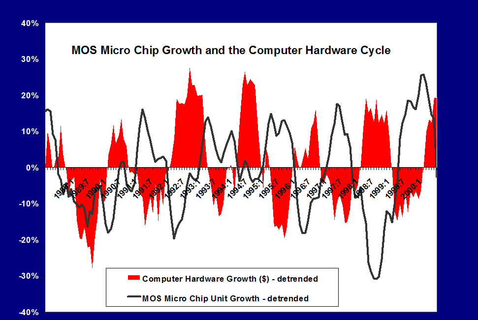
Here is an exhibit I prepared in 2000 for a magazine serving the printed circuit board industry.

semicycle

The data come from two sources – the Semiconductor Industry Association (SIA) World Semiconductor Trade Statistics database and the Census Bureau manufacturing series for computer equipment.

This sort of analytics spawned a spate of academic research, beginning more or less with the work of Tan and Mathews in Australia.

One of my favorites is a working paper released by DRUID – the Danish Research Unit for Industrial Dynamics called Cyclical Dynamics in Three Industries. Tan and Mathews consider cycles in semiconductors, computers, and what they call the flat panel display industry. They start with quoting “industry experts” and, specifically, some of my work with Economic Data Resources on the computer (PC) cycle. These researchers went on to publish in the Journal of Business Research and Technological Forecasting and Social Change in 2010. A year later in 2011, Tan published an interesting article on the sequencing of cyclical dynamics in semiconductors.

Essentially, the appearance of cycles and what I have called quasi-cycles or pseudo-cycles in the semiconductor industry and other IT categories, like computers, result from the interplay of innovation, investment, and pricing. In semiconductors, for example, Moore’s law – which everyone always predicts will fail at some imminent future point – indicates that continuing miniaturization will lead to periodic reductions in the cost of information processing. At some point in the 1980’s, this cadence was firmly established by introductions of new microprocessors by Intel roughly every 18 months. The enhanced speed and capacity of these microprocessors – the “central nervous system” of the computer – was complemented by continuing software upgrades, and, of course, by the movement to graphical interfaces with Windows and the succession of Windows releases.

Back along the supply chain, semiconductor fabs were retooling periodically to produce chips with more and more transitors per volume of silicon. These fabs were, simply put, fabulously expensive and the investment dynamics factors into pricing in semiconductors. There were famous gluts, for example, of memory chips in 1996, and overall the whole IT industry led the recession of 2001 with massive inventory overhang, resulting from double booking and the infamous Y2K scare.

Statistical Modeling of IT Cycles

A number of papers, summarized in Aubrey deploy VAR (vector autoregression) models to capture leading indicators of global semiconductor sales. A variant of these is the Bayesian VAR or BVAR model. Basically, VAR models sort of blindly specify all possible lags for all possible variables in a system of autoregressive models. Of course, some cutoff point has to be established, and the variables to be included in the VAR system have to be selected by one means or another. A BVAR simply reduces the number of possibilities by imposing, for example, sign constraints on the resulting coefficients, or, more ambitiously, employs some type of prior distribution for key variables.

Typical variables included in these models include:

  • WSTS monthly semiconductor shipments (now by subscription only from SIA)
  • Philadelphia semiconductor index (SOX) data
  • US data on various IT shipments, orders, inventories from M3
  • data from SEMI, the association of semiconductor equipment manufacturers

Another tactic is to filter out low and high frequency variability in a semiconductor sales series with something like the Hodrick-Prescott (HP) filter, and then conduct a spectral analysis.

Does the Semiconductor/Computer/IT Cycle Still Exist?

I wonder whether academic research into IT cycles is a case of “redoubling one’s efforts when you lose sight of the goal,” or more specifically, whether new configurations of forces are blurring the formerly fairly cleanly delineated pulses in sales growth for semiconductors, computers, and other IT hardware.

“Hardware” is probably a key here, since there have been big changes since the 1990’s and early years of this brave new century.

For one thing, complementarities between software and hardware upgrades seem to be breaking down. This began in earnest with the development of virtual servers – software which enabled many virtual machines on the same hardware frame, in part because the underlying circuitry was so massively powerful and high capacity now. Significant declines in the growth of sales of these machines followed on wide deployment of this software designed to achieve higher efficiencies of utilization of individual machines.

Another development is cloud computing. Running the data side of things is gradually being taken away from in-house IT departments in companies and moved over to cloud computing services. Of course, critical data for a company is always likely to be maintained in-house, but the need for expanding the number of big desktops with the number of employees is going away – or has indeed gone away.

At the same time, tablets, Apple products and Android machines, created a wave of destructive creation in people’s access to the Internet, and, more and more, for everyday functions like keeping calendars, taking notes, even writing and processing photos.

But note – I am not studding this discussion with numbers as of yet.

I suspect that underneath all this change it should be possible to identify some IT invariants, perhaps in usage categories, which continue to reflect a kind of pulse and cycle of activity.

Prospects for the 2nd Quarter 2014 and the Rest of the Year

Well, it’s the first day of the 3rd quarter 2014, and time to make an assessment of what happened in Q2 and also what is likely to transpire the rest of the year.

The Big Write-Down

Of course, the 1st quarter 2014 numbers were surprisingly negative – and almost no one saw that coming. Last Wednesday (June 25) the Bureau of Economic Analysis (BEA) revised last estimates of 1st quarter real GDP down a -2.9 percent decrease on a quarter-by-quarter basis.

The Accelerating Growth Meme

Somehow media pundits and the usual ranks of celebrity forecasters seem heavily invested in the “accelerating growth” meme in 2014.

Thus, in mid-June Mark Zandi of Moody’s tries to back up Moody’s Analytics U.S. Macro Forecast calling for accelerating growth the rest of the year, writing,

The economy’s strength is increasingly evident in the job market. Payroll employment rose to a new high in May as the U.S. finally replaced all of the 8.7 million jobs lost during the recession, and job growth has accelerated above 200,000 per month since the start of the year. The pace of job creation is almost double that needed to reduce unemployment, even with typical labor force gains. More of the new positions are also better paying than was the case earlier in the recovery.

After the BEA released its write-down numbers June 25, the Canadian Globe and Mail put a happy face on everything, writing that The US Economy is Back on Track since,

Hiring, retail sales, new-home construction and consumer confidence all rebounded smartly this spring. A separate government report Wednesday showed inventories for non-defense durable goods jumped 1 per cent in May after a 0.4-per-cent increase the previous month.

Forecasts for the Year Being Cut-Back

On the other hand, the International Monetary Fund (IMF) cut its forecast for US growth,

In its annual review of the U.S. economy, the IMF cut its forecast for U.S. economic growth this year by 0.8 percentage point to 2%, citing a harsh winter, a struggling housing market and weak international demand for the country’s products.

Some Specifics

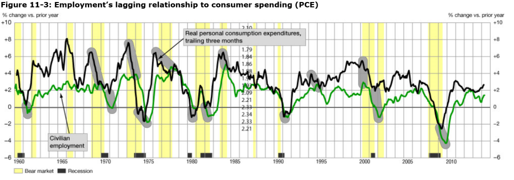
The first thing to understand in this context is that employment is usually a lagging indicator of the business cycle. Ahead of the Curve makes this point dramatically with the following chart.

employment

The chart shows employment change and growth lag changes in the business cycle. Thus, note that the green line peaks after growth in personal consumption expenditures in almost every case, where these growth rates are calculated on a year-over-year basis.

So Zandi’s defense of the Moody’s Analytics accelerating growth forecast for the rest of 2014 has to be taken with a grain of salt.

It really depends on other things – whether for example, retail sales are moving forward, what’s happening in the housing market (to new-home construction and other variables), also to inventories and durable goods spending. Also have exports rebounded, and imports (a subtraction from GDP) been reined in?

Retail Sales

If there is going to be accelerating economic growth, consumer demand, which certainly includes retail sales, has to improve dramatically.

However, the picture is mixed with significant rebound in sales in April, but lower-than-expected retail sales growth in May.

Bloomberg’s June take on this is in an article Cooling Sales Curb Optimism on U.S. Growth Rebound: Economy.

The US Census report estimates U.S. retail and food services sales for May, adjusted for seasonal variation and holiday and trading-day differences, but not for price changes, were $437.6 billion, an increase of 0.3 percent (±0.5)* from the previous month.

Durable Goods Spending

In the Advance Report on Durable Goods Manufacturers’ Shipments, Inventories and Orders May 2014 we learn that,

New orders for manufactured durable goods in May decreased $2.4 billion or 1.0 percent to $238.0 billion, the U.S. Census Bureau announced today.

On the other hand,

Shipments of manufactured durable goods in May, up four consecutive months, increased $0.6 billion or 0.3 percent to $238.6 billion

Of course, shipments are a lagging indicator of the business cycle.

Finally, inventories are surging –

Inventories of manufactured durable goods in May, up thirteen of the last fourteen months, increased $3.8 billion or 1.0 percent to $397.8 billion. This was at the highest level since the series was first published on a NAICS basis and followed a 0.3 percent April increase.

Inventory accumulation is a coincident indicator (in a negative sense) of the business cycle, according to NBER documents.

New Home Construction

From the Joint Release U.S. Department of Housing and Urban Development,

Privately-owned housing units authorized by building permits in May were at a seasonally adjusted annual rate of 991,000. This is 6.4 percent (±0.8%) below the revised April rate of 1,059,000 and is 1.9 percent (±1.4%) below the May 2013 estimate of 1,010,000…

Privately-owned housing starts in May were at a seasonally adjusted annual rate of 1,001,000. This is 6.5 percent (±10.2%)* below the

revised April estimate of 1,071,000, but is 9.4 percent (±11.0%)* above the May 2013 rate of 915,000.

Single-family housing starts in May were at a rate of 625,000; this is 5.9 percent (±12.7%)* below the revised April figure of 664,000.

No sign of a rebound in new home construction in these numbers.

Exports and Imports

The latest BEA report estimates,

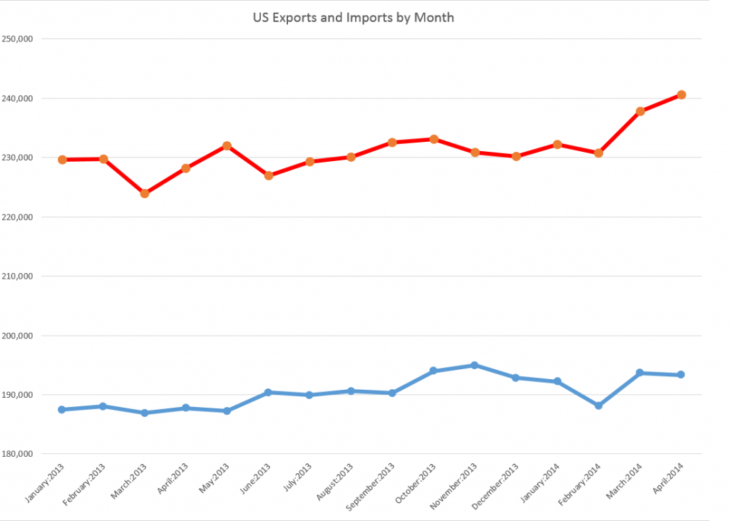
April exports were $0.3 billion less than March exports of $193.7 billion. April imports were $2.7 billion more than March imports of $237.8 billion

Here is a several month perspective.

XM

Essentially, the BEA trade numbers suggest the trade balance deteriorated March to April with a sharp uptick in imports and a slight drop in exports.

Summary

Well, it’s not a clear picture. The economy is teetering on the edge of a downturn, which it may still escape.

Clearly, real growth in Q2 has to be at least 2.9 percent in order to counterbalance the drop in Q1, or else the first half of 2014 will show a net decrease.

CNN offers this with an accompanying video

Goldman Sachs economists trimmed second quarter tracking GDP to 3.5 percent from 4.1 percent, and Barclays economists said tracking GDP for the second quarter fell to 2.9 percent from 4 percent. At a pace below 3 percent, the economy could show contraction for the first half due to the steep first quarter decline of 2.9 percent.

top picture http://www.bbc.com/news/magazine-24045598